Download & Play with Cryptocurrencies Historical Data in Python
To access the CryptoCompare public API in Python, we can use the following Python wrapper available on GitHub: cryCompare.
%load_ext autoreload
%autoreload 2

import numpy as np
import pandas as pd
from joblib import Parallel, delayed
import operator
import matplotlib.pyplot as plt

from crycompare import *

from ClusterLib.clusterlib import *
from ClusterLib.distlib import *

%matplotlib inline
With the coinList() function we can fetch all the available cryptocurrencies (about 1450).
p = Price()

coinList = p.coinList()
coins = sorted(list( coinList['Data'].keys() ))
With the histoDay() function we can fetch the historical data (OHLC prices and volumes) for a given pair. We keep only coins which have a non-trivial history (about 1350).
h = History()

df_dict = {}
for coin in coins:
    histo = h.histoDay(coin,'USD',allData=True)
    if histo['Data']:
        df_histo = pd.DataFrame(histo['Data'])
        df_histo['time'] = pd.to_datetime(df_histo['time'],unit='s')
        df_histo.index = df_histo['time']
        del df_histo['time']
        del df_histo['volumefrom']
        del df_histo['volumeto']

        df_dict[coin] = df_histo
We store all info in a dataframe with 2-level columns: the first level contains the coin names, the second one, the OHLC prices.
crypto_histo = pd.concat(df_dict.values(), axis=1, keys=df_dict.keys())
histo_coins = [elem for elem in crypto_histo.columns.levels[0] if not elem == 'MYC']
Since many coins are quite recent, many have relatively short time series of historical data. We sort them by the decreasing length of their time series. BTC (Bitcoin) has the longest one, as expected.
histo_length = {}
for coin in histo_coins:
    histo_length[coin] = np.sum( ~np.isnan(crypto_histo[coin]['close'].values) )

sorted_length = sorted(histo_length.items(), key=operator.itemgetter(1),reverse=True)
For the following, we will only consider the 300 longest time series.
# we keep the 300 coins having the longest time series of historical prices
sub_coins = [sorted_length[i][0] for i in range(300)]

sub_crypto_histo = crypto_histo[sub_coins]
sub_crypto_histo.tail()
| POT | TEK | BTC | ... | DGD | PIGGY | DIEM | |||||||||||||||
|---|---|---|---|---|---|---|---|---|---|---|---|---|---|---|---|---|---|---|---|---|---|
| close | high | low | open | close | high | low | open | close | high | ... | low | open | close | high | low | open | close | high | low | open | |
| time | |||||||||||||||||||||
| 2017-08-21 | 0.1282 | 0.1368 | 0.1265 | 0.1321 | 0.000120 | 0.000451 | 0.000079 | 0.000122 | 4005.10 | 4097.25 | ... | 74.14 | 78.93 | 0.000681 | 0.000696 | 0.000555 | 0.000610 | 0.000040 | 0.000041 | 0.000040 | 0.000041 |
| 2017-08-22 | 0.1267 | 0.1411 | 0.1089 | 0.1282 | 0.000123 | 0.000166 | 0.000108 | 0.000120 | 4089.70 | 4142.68 | ... | 67.84 | 78.34 | 0.000614 | 0.000704 | 0.000397 | 0.000681 | 0.000041 | 0.000041 | 0.000036 | 0.000040 |
| 2017-08-23 | 0.1245 | 0.1335 | 0.1191 | 0.1267 | 0.000124 | 0.000170 | 0.000081 | 0.000123 | 4141.09 | 4255.62 | ... | 76.57 | 78.85 | 0.000621 | 0.000809 | 0.000570 | 0.000614 | 0.000041 | 0.000043 | 0.000041 | 0.000041 |
| 2017-08-24 | 0.1289 | 0.1324 | 0.1211 | 0.1245 | 0.000130 | 0.000131 | 0.000082 | 0.000124 | 4318.35 | 4364.11 | ... | 80.01 | 89.70 | 0.000648 | 0.000698 | 0.000576 | 0.000621 | 0.000043 | 0.000044 | 0.000041 | 0.000041 |
| 2017-08-25 | 0.1335 | 0.1576 | 0.1266 | 0.1289 | 0.000133 | 0.000179 | 0.000086 | 0.000130 | 4442.46 | 4461.71 | ... | 90.69 | 93.97 | 0.000622 | 0.000669 | 0.000602 | 0.000648 | 0.000044 | 0.000045 | 0.000043 | 0.000043 |
5 rows × 1200 columns
All these 300 time series have at least 1000 days of observed prices. We will only consider these days for the correlation study.
N = len(sub_coins)
recent_histo = sub_crypto_histo[-1000:]
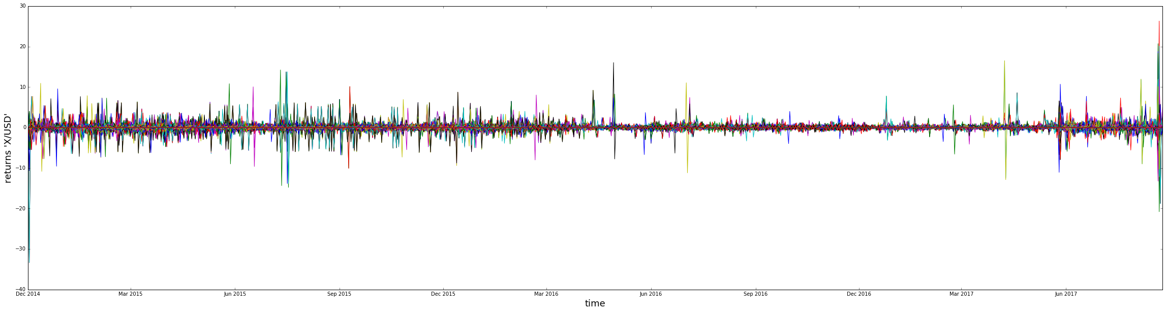
Below, we compute their daily log-returns.
returns_dict = {}
for coin in sub_coins:
    coin_histo = recent_histo[coin]
    coin_returns = pd.DataFrame(np.diff(np.log(coin_histo.get_values()),axis=0))
    returns_dict[coin] = coin_returns

recent_returns = pd.concat(returns_dict.values(),axis=1,keys=returns_dict.keys())
recent_returns.index = recent_histo.index[1:]
recent_returns = recent_returns.replace([np.inf, -np.inf], np.nan)
recent_returns = recent_returns.fillna(value=0)
recent_returns.isnull().values.any()
False
plt.figure(figsize=(40,10))
for coin in sub_coins:
    plt.plot(recent_returns[coin])
#plt.legend(sub_coins,loc='upper left')
plt.xlabel('time',fontsize=18)
plt.ylabel('returns \'X/USD\'',fontsize=18)
plt.show()
Notice below that the scale is pretty huge compared to other financial assets (which are usually contained in a (-0.15,0.15) range, with some tails valued at ~2 or 3).
Now, we compute a correlation/distance matrix between all these coins. Notice that we consider here the OHLC representation, and thus we have to compute a correlation between random vectors, and not random variables (which is usually done by considering only the ‘close’ price for example). The distance correlation is a relevant measure of statistical dependence for that purpose. We apply it between the 300x299/2 = 44850 pairs in parallel using the joblib library.
dist_mat = np.zeros((N,N))
a,b = np.triu_indices(N,k=1)
dist_mat[a,b] = Parallel(n_jobs=-2,verbose=1) (delayed(distcorr)(recent_returns[sub_coins[a[i]]],recent_returns[sub_coins[b[i]]]) for i in range(len(a)))
dist_mat[b,a] = dist_mat[a,b]
[Parallel(n_jobs=-2)]: Done 39186 tasks      | elapsed: 19.3min
[Parallel(n_jobs=-2)]: Done 42036 tasks      | elapsed: 20.7min
[Parallel(n_jobs=-2)]: Done 44850 out of 44850 | elapsed: 22.1min finished
Then, using the dendrogram obtained from the Ward hierarchical clustering method, we can sort the coins so that their correlation/distance matrix is more readable.
seriated_dist_mat, res_order, res_linkage = compute_serial_matrix(dist_mat)
ordered_coins = [sub_coins[res_order[i]] for i in range(len(res_order))]
plt.figure(figsize=(80,80))
plt.pcolormesh(seriated_dist_mat)
#plt.colorbar()
plt.xlim([0,N])
plt.ylim([0,N])
plt.xticks( np.arange(N)+0.5, ordered_coins, rotation=90, fontsize=25 )
plt.yticks( np.arange(N)+0.5, ordered_coins, fontsize=25 )
plt.show()
We can observe that some coins do cluster together as they are correlated and uncorrelated to the rest of the coins in a similar way.
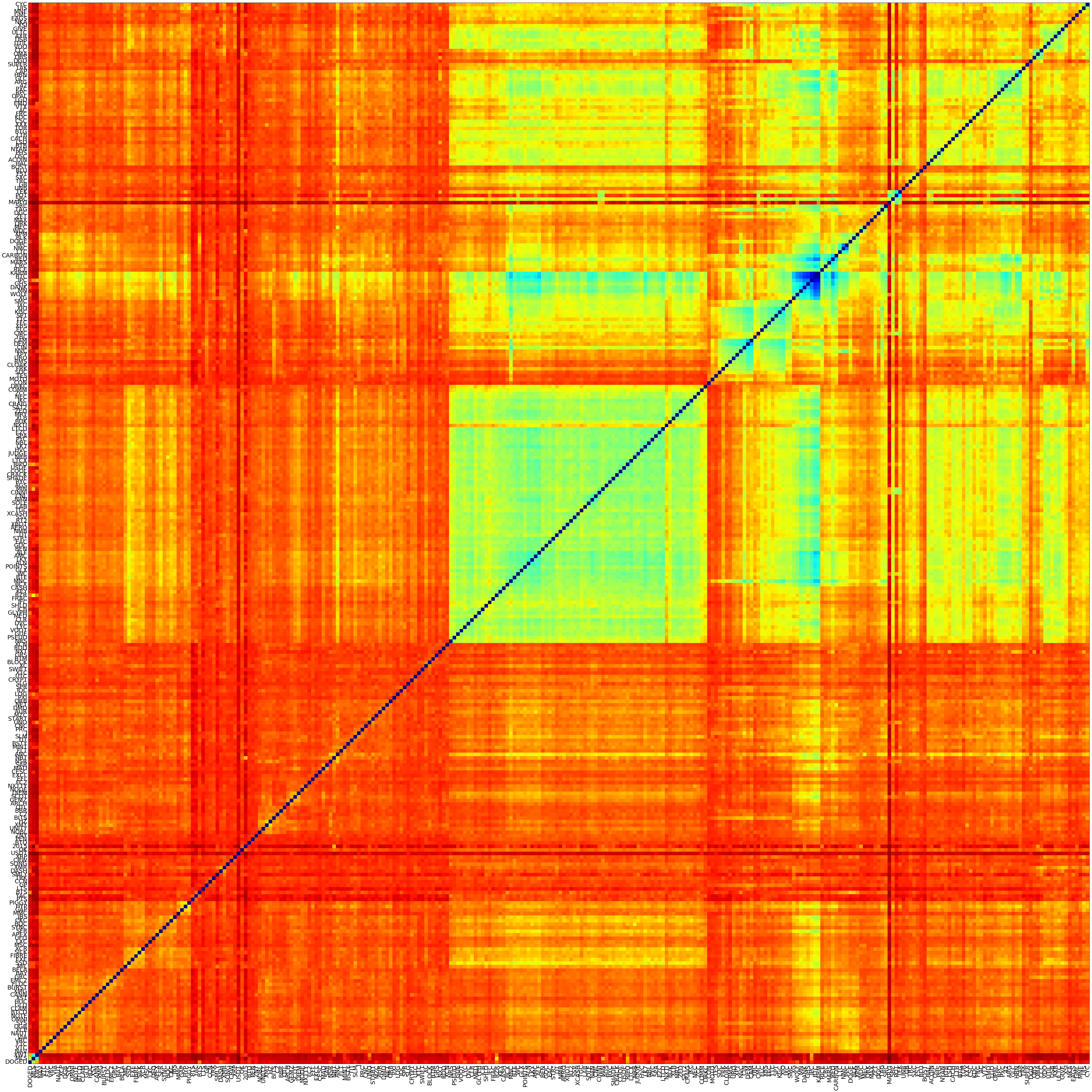
For example, we obtain the following clusters (if we ask for 30 groups).
nb_clusters = 30

cluster_map = pd.DataFrame(scipy.cluster.hierarchy.fcluster(res_linkage,nb_clusters,'maxclust'),index=ordered_coins)
clusters = []
k = 0
for i in range(0,nb_clusters):
    compo = cluster_map[cluster_map[0]==(i+1)].index.values
    clusters.append(compo)
    k = k + len(compo)
for cluster in clusters:
    print(cluster)
['GEMZ' 'MINT' 'NMC']
['BTCD' 'MIL' 'SFR' 'TRK' 'FC2' 'AUR' 'ALN' 'LKY' 'CLOAK' 'URO' 'YBC' 'XPM'
'EMD']
['PIGGY' 'PEN' 'C2' 'DMD' 'POINTS' 'XLB' 'RMS' 'AC' 'VDO' 'AXR' 'XSI']
['LXC' 'XMY' 'PSEUD' 'GUE' 'LK7' 'SAT2']
['UFO' 'HZ' 'NSR' 'UNO' 'SLG' 'GRS' 'AMC' 'SPA' 'MRY']
['ACOIN' 'RPC' 'DSB' 'UIS']
['XMR' 'NRS' 'OPAL']
['DGC' 'CACH' 'XXX' 'DGD']
['OMNI' 'QTL' 'NODE' 'BLK' 'LTB' 'ULTC']
['LTC' 'MEC']
['HUC' 'CANN' 'NBT']
['TAG']
['EMC2' 'CRAIG' 'CSC' '42' 'HBN' 'CAP' 'EAGS' 'GML']
['FLT' 'TEK' 'GB' 'SXC' 'BLU' 'TOR' 'KDC' 'GLC' 'CYC']
['NAUT' 'XCP' 'EXE']
['ZNY' 'BITS' 'SAR' 'ANC' 'GLX' 'PYC' 'OSC']
['SYS' 'BURST' 'HYP' 'PTS' 'OK' 'EXCL' 'IFC' 'KEY' 'XBOT' 'VTX' 'SUPER']
['NOBL' 'EFL' 'CESC' 'BSTY' 'CASH' 'USDE' 'RED']
['CRW' 'GLYPH' 'NRB' 'DEM' 'LSD' 'FRC' 'PXC' 'ARG' 'UTIL']
['VTC' 'XST' 'FLDC' 'BAY' 'BELA' 'FIBRE' 'CKC' 'GAP' 'BTS' 'LTS' 'CCN'
'SMLY' 'BTQ' 'SCOT' 'START' 'MZC' 'ORB' 'PXI' 'LOG' 'IOC' 'CRYPT' 'XC'
'BTM' 'XCN' 'LYC' 'DVC' 'CLR' 'MED' 'FRAC' 'STR*' 'DT' 'NMB' 'TGC' 'NAN'
'CNL' 'AGS' 'SHADE' 'CRACK' 'LTCX' 'HVC' 'EZC' 'LTCD' 'NXTI' 'BUK' 'JKC'
'ZCC' 'COMM' 'DRKC' 'CON' 'MOTO' 'SDC' 'FRK' 'XPY' 'CIN' 'CAM' 'CMC' 'ELC'
'XBS' 'FFC' 'TTC' 'SPT' 'KGC' 'XJO' 'IXC' 'SMC' 'XG' 'DANK' 'GHS' 'IPC'
'KARM' 'CRC' 'MARS' 'CARBON']
['SILK' 'WC' 'MAX']
['NAV' 'CLAM' 'MSC' 'APEX' 'BQC' 'MMC' 'SONG' 'PRC' 'CNC' 'VOOT' 'MNC'
'SSV' 'XCASH' 'SOLE' 'NBL' 'NVC' 'PPC' 'DOGE' 'SRC' 'TRC' 'OBS']
['XWT' 'FTC' 'NOTE' 'GLD' 'XCR' 'XRP' 'USDT' 'DIEM' 'WDC' 'MARYJ' 'BOST'
'HAL' 'NYAN']
['VRC' 'VIA' 'DGB' 'DASH' 'BBR' 'SLM']
['XMG' 'SSD' 'JBS' 'GP' 'MAD' 'J' 'SWIFT' 'NEC']
['DOGED' 'MLS' 'SYNC' 'TIT']
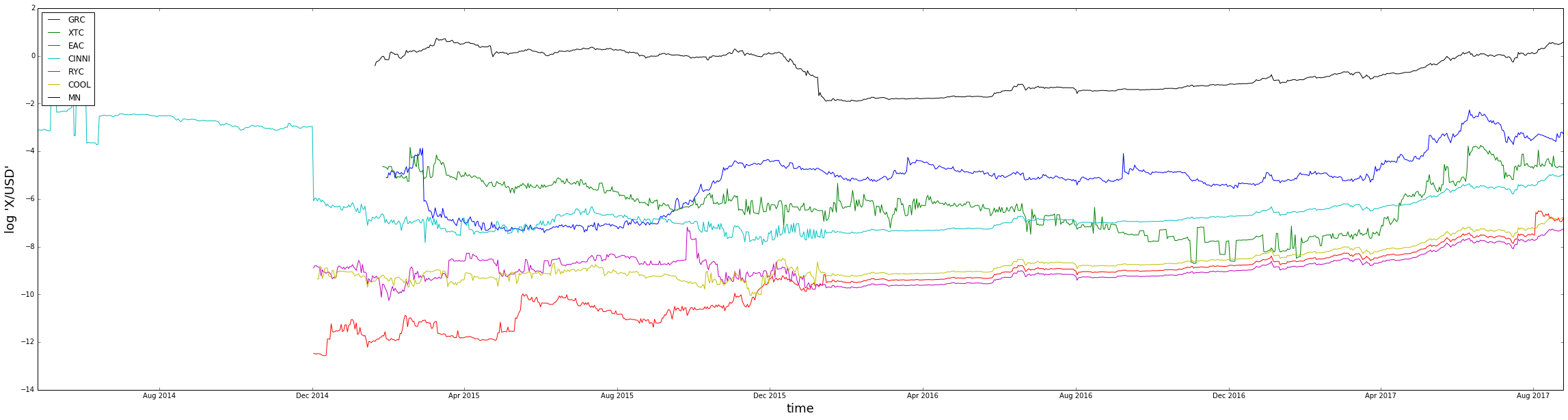
['GRC' 'XTC' 'EAC' 'CINNI' 'RYC' 'COOL' 'MN']
['YAC' '2015' 'UNITY' 'ARCH' 'NXTTY' 'NET' 'SPR' 'UTC' 'BLOCK' 'NXT' 'RDD'
'ICB' 'SHLD' 'RZR' 'BCX' 'BTE' 'ALF' 'BEN' 'GDC' 'AERO' 'RT2' 'LAB' 'MIN'
'RIPO' 'JUDGE' 'ZED' 'TES' 'BTC' 'RICE']
['LGD' 'TAK' 'CCC' 'MNE']
['WOLF' 'QRK' 'ZET' 'SBC' 'POT' 'UNB' 'FST' 'PHS' 'BTB' 'BTG' 'OMA' 'GIVE'
'NKA']
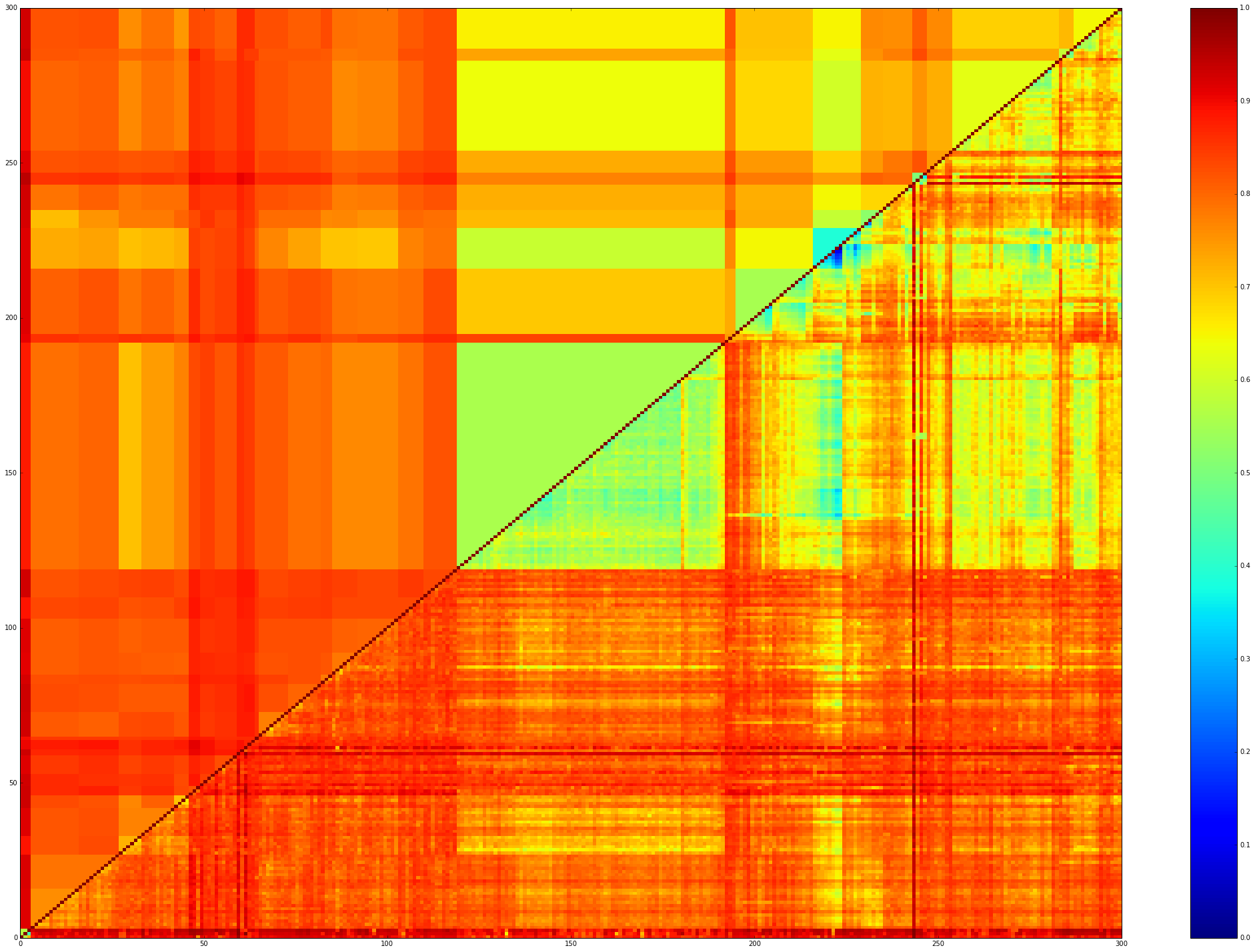
We can use these clusters to average the values of the correlation-distances inside and in-between the clusters. We obtain the following filtered matrix:
display_filtered_distances_using_clusters(seriated_dist_mat,clusters)
For example, below are the ‘close’ log-prices of one rather strong cluster:
plt.figure(figsize=(40,10))
alt_coins = ['GRC', 'XTC', 'EAC', 'CINNI', 'RYC', 'COOL', 'MN']
for coin in alt_coins:
    plt.plot(np.log(sub_crypto_histo[coin]['close']))
plt.xlabel('time',fontsize=18)
plt.ylabel('log \'X/USD\'',fontsize=18)
plt.legend(alt_coins,loc='upper left')
plt.show()