Ether vs. Bitcoin -- Part 0
In this introduction notebook, we simply displayed the distribution of the returns and see that tails are heavy, meaning that standard quant models cannot be applied to cryptocurrencies either…
import numpy as np
import scipy
import pandas as pd
import matplotlib.pyplot as plt
%matplotlib inline
import seaborn as sns
We load historical data for ETH/USD and BTC/USD prices into pandas dataframe:
histo_BTC = pd.read_csv('BTCUSDT.csv')
histo_ETH = pd.read_csv('ETHUSDT.csv')
We convert the time in seconds of the ‘date’ column into dates:
histo_ETH['date'] = pd.to_datetime(histo_ETH['date'],unit='s')
histo_BTC['date'] = pd.to_datetime(histo_BTC['date'],unit='s')
We take a look at the dataframes, we display the tail and head of the dataframe for ETH/USD prices:
histo_ETH.tail()
| date | high | low | open | close | volume | quoteVolume | weightedAverage | |
|---|---|---|---|---|---|---|---|---|
| 32805 | 2017-06-21 16:30:00 | 330.00000 | 326.000000 | 327.953902 | 330.00000 | 176417.191868 | 537.719509 | 328.084046 |
| 32806 | 2017-06-21 17:00:00 | 330.00000 | 323.415775 | 330.000000 | 325.99900 | 235115.812230 | 721.174679 | 326.017841 |
| 32807 | 2017-06-21 17:30:00 | 325.99900 | 309.700000 | 325.999000 | 314.00000 | 1600835.815479 | 5082.966612 | 314.941242 |
| 32808 | 2017-06-21 18:00:00 | 321.49800 | 310.986006 | 314.000000 | 317.00007 | 636047.132561 | 2016.865421 | 315.364191 |
| 32809 | 2017-06-21 18:30:00 | 330.01475 | 317.001070 | 319.100000 | 323.05000 | 379339.250364 | 1165.505294 | 325.471924 |
histo_ETH.head()
| date | high | low | open | close | volume | quoteVolume | weightedAverage | |
|---|---|---|---|---|---|---|---|---|
| 0 | 2015-08-08 06:00:00 | 1.85 | 1.61 | 1.65 | 1.85 | 90.024655 | 53.0404 | 1.697286 |
| 1 | 2015-08-08 06:30:00 | 1.85 | 1.71 | 1.85 | 1.71 | 20.686119 | 12.0898 | 1.711040 |
| 2 | 2015-08-08 07:00:00 | 1.85 | 0.50 | 1.75 | 1.85 | 33.717419 | 18.8862 | 1.785290 |
| 3 | 2015-08-08 07:30:00 | 1.85 | 1.85 | 1.85 | 1.85 | 0.000000 | 0.0000 | 1.850000 |
| 4 | 2015-08-08 08:00:00 | 1.85 | 1.85 | 1.85 | 1.85 | 0.000000 | 0.0000 | 1.850000 |
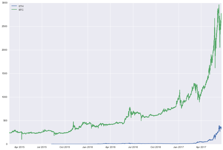
Below, we display their price time series:
plt.figure(figsize=(15,10))
plt.plot(histo_ETH['date'],histo_ETH['close'])
plt.plot(histo_BTC['date'],histo_BTC['close'])
plt.legend(['ETH','BTC'],loc=0)
plt.show()
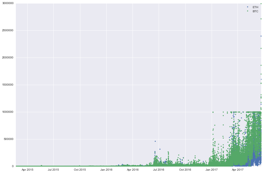
And the volumes traded for the two crypto/USD rates:
plt.figure(figsize=(15,10))
plt.plot(histo_ETH['date'],histo_ETH['volume'],'.')
plt.plot(histo_BTC['date'],histo_BTC['volume'],'.')
plt.legend(['ETH','BTC'],loc=0)
plt.show()
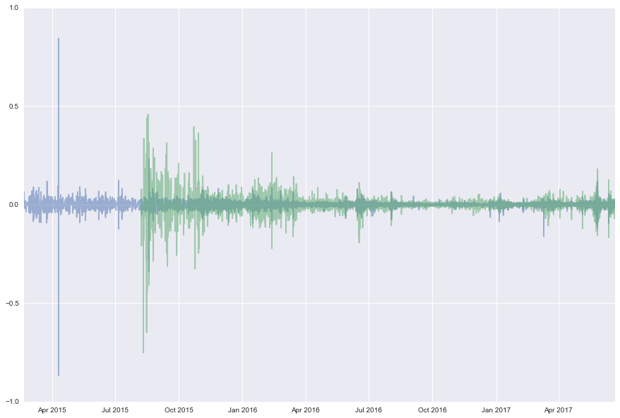
We can also compute the returns for ETH/USD and BTC/USD:
returns_BTC = pd.DataFrame(np.diff(np.log(histo_BTC['close'].get_values()),axis=0))
returns_BTC.index = histo_BTC['date'].get_values()[1:]
returns_BTC.columns = ['returns']

returns_ETH = pd.DataFrame(np.diff(np.log(histo_ETH['close'].get_values()),axis=0))
returns_ETH.index = histo_ETH['date'].get_values()[1:]
returns_ETH.columns = ['returns']
And we display them:
plt.figure(figsize=(15,10))
plt.plot(returns_BTC,alpha=0.5)
plt.plot(returns_ETH,alpha=0.5)
plt.show()
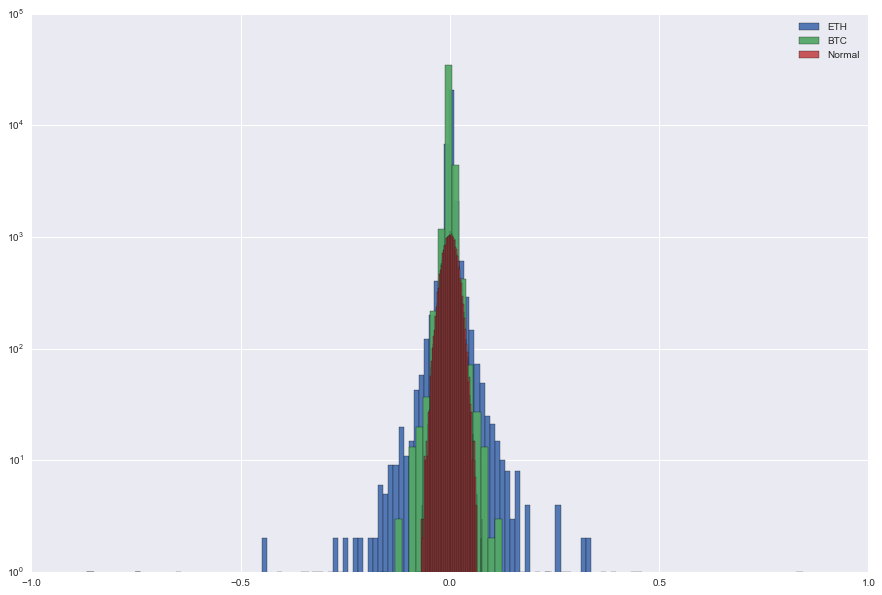
We can also display the distribution of their returns. We display them alongside the Gaussian distribution. We can see that both ETH/USD and BTC/USD returns are heavy-tailed! Be careful of when using standard quant models and value-at-risks.
plt.figure(figsize=(15,10))
x = np.random.normal(0,np.std(returns_ETH['returns']),len(returns_ETH['returns']))
plt.hist(returns_ETH['returns'],bins=100,log=True,alpha=0.95)
plt.hist(returns_BTC['returns'],bins=100,log=True,alpha=0.95)
plt.hist(x,bins=100,log=True,alpha=0.95)
plt.legend(['ETH','BTC','Normal'])
plt.show()