Ether vs. Bitcoin -- Part 0 bis
For the last few days, ETH has lost 1/3 of its value with -20% several days in a row. We update the initial study with up-to-date data to take into account this recent drawback. We add a comment on the skewness of the returns distribution at the end.
import numpy as np
import scipy
import pandas as pd
import matplotlib.pyplot as plt
%matplotlib inline
import seaborn as sns
We load historical data for ETH/USD and BTC/USD prices into pandas dataframe:
histo_BTC = pd.read_csv('BTCUSDT_1.csv')
histo_ETH = pd.read_csv('ETHUSDT_1.csv')
We convert the time in seconds of the ‘date’ column into dates:
histo_ETH['date'] = pd.to_datetime(histo_ETH['date'],unit='s')
histo_BTC['date'] = pd.to_datetime(histo_BTC['date'],unit='s')
We take a look at the dataframes, we display the tail and head of the dataframe for ETH/USD prices:
histo_ETH.tail()
| date | high | low | open | close | volume | quoteVolume | weightedAverage | |
|---|---|---|---|---|---|---|---|---|
| 33122 | 2017-06-28 07:00:00 | 273.340000 | 266.5 | 266.500000 | 271.000000 | 787049.632584 | 2911.991623 | 270.278811 |
| 33123 | 2017-06-28 07:30:00 | 276.280002 | 270.0 | 270.000070 | 276.280002 | 460955.337537 | 1680.342777 | 274.322206 |
| 33124 | 2017-06-28 08:00:00 | 280.280070 | 275.0 | 276.280002 | 280.000000 | 586820.959374 | 2114.449571 | 277.528945 |
| 33125 | 2017-06-28 08:30:00 | 280.279000 | 268.6 | 280.100000 | 276.525969 | 833818.197678 | 3043.753814 | 273.944034 |
| 33126 | 2017-06-28 09:00:00 | 280.754655 | 276.4 | 276.525969 | 279.144106 | 515923.390002 | 1846.289433 | 279.437980 |
histo_ETH.head()
| date | high | low | open | close | volume | quoteVolume | weightedAverage | |
|---|---|---|---|---|---|---|---|---|
| 0 | 2015-08-08 06:00:00 | 1.85 | 1.61 | 1.65 | 1.85 | 90.024655 | 53.0404 | 1.697286 |
| 1 | 2015-08-08 06:30:00 | 1.85 | 1.71 | 1.85 | 1.71 | 20.686119 | 12.0898 | 1.711040 |
| 2 | 2015-08-08 07:00:00 | 1.85 | 0.50 | 1.75 | 1.85 | 33.717419 | 18.8862 | 1.785290 |
| 3 | 2015-08-08 07:30:00 | 1.85 | 1.85 | 1.85 | 1.85 | 0.000000 | 0.0000 | 1.850000 |
| 4 | 2015-08-08 08:00:00 | 1.85 | 1.85 | 1.85 | 1.85 | 0.000000 | 0.0000 | 1.850000 |
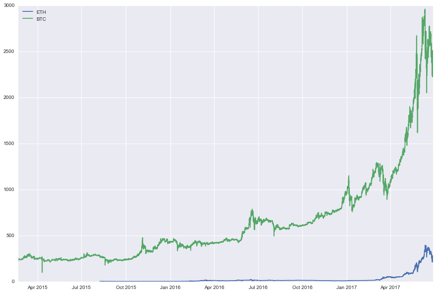
Below, we display their price time series:
plt.figure(figsize=(15,10))
plt.plot(histo_ETH['date'],histo_ETH['close'])
plt.plot(histo_BTC['date'],histo_BTC['close'])
plt.legend(['ETH','BTC'],loc=0)
plt.show()
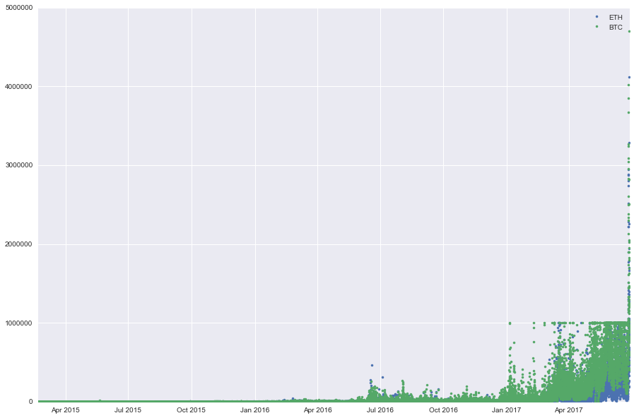
And the volumes traded for the two crypto/USD rates:
plt.figure(figsize=(15,10))
plt.plot(histo_ETH['date'],histo_ETH['volume'],'.')
plt.plot(histo_BTC['date'],histo_BTC['volume'],'.')
plt.legend(['ETH','BTC'],loc=0)
plt.show()
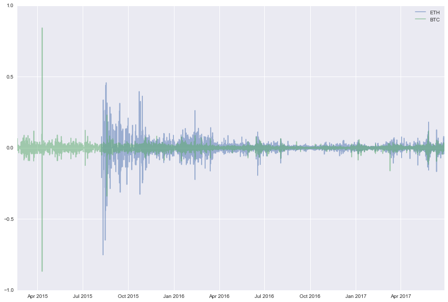
We can also compute the returns for ETH/USD and BTC/USD:
returns_BTC = pd.DataFrame(np.diff(np.log(histo_BTC['close'].get_values()),axis=0))
returns_BTC.index = histo_BTC['date'].get_values()[1:]
returns_BTC.columns = ['returns']

returns_ETH = pd.DataFrame(np.diff(np.log(histo_ETH['close'].get_values()),axis=0))
returns_ETH.index = histo_ETH['date'].get_values()[1:]
returns_ETH.columns = ['returns']
And we display them:
plt.figure(figsize=(15,10))
plt.plot(returns_ETH,alpha=0.5)
plt.plot(returns_BTC,alpha=0.5)
plt.legend(['ETH','BTC'],loc=0)
plt.show()
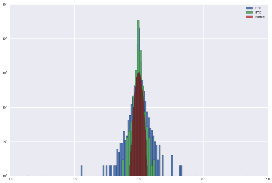
We can also display the distribution of their returns. We display them alongside the Gaussian distribution. We can see that both ETH/USD and BTC/USD returns are heavy-tailed! Be careful of when using standard quant models and value-at-risks.
plt.figure(figsize=(15,10))
x = np.random.normal(0,np.std(returns_ETH['returns']),len(returns_ETH['returns']))
plt.hist(returns_ETH['returns'],bins=100,log=True,alpha=0.95)
plt.hist(returns_BTC['returns'],bins=100,log=True,alpha=0.95)
plt.hist(x,bins=100,log=True,alpha=0.95)
plt.legend(['ETH','BTC','Normal'])
plt.show()
Now that we have shown that the distribution of returns are heavy-tailed, we want to look at the skewness, i.e. the asymmetry of the distribution.
The normal distribution has a skewness of 0 since it is symmetric. We can verify it:
scipy.stats.skew(x)
0.021692662768936662
For ETH and BTC we have respectively a skewness of:
scipy.stats.skew(returns_ETH['returns']), scipy.stats.skew(returns_BTC['returns'])
(-2.6956406272458073, -2.168724435124142)
They are both negatively skewed, that means a greater chance of extremely negative outcomes for investors in these cryptocurrencies.