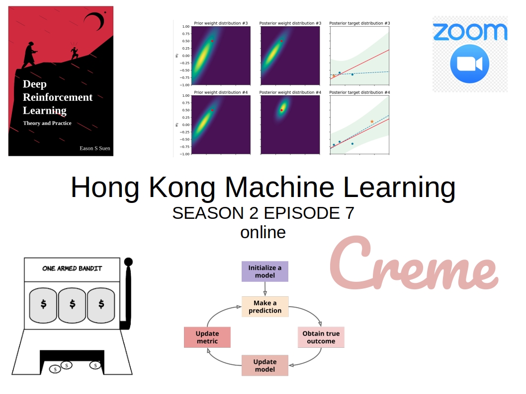
[HKML] Hong Kong Machine Learning Meetup Season 2 Episode 7
[HKML] Hong Kong Machine Learning Meetup Season 2 Episode 7
When?
- Wednesday, June 10, 2020 from 7:00 PM to 9:00 PM
Where?
- At your home, on zoom. All meetups will be online as long as this COVID-19 crisis is not over.
Thanks to our patrons for supporting the meetup!
Check the patreon page to join the current list:
Programme:
Max Halford - A brief introduction to online machine learning
Online learning algorithms are usually much less well-known than their batch counterparts: For example, the estimation of mean, variance, and covariance.
Max is developing a library, Creme, available on GitHub, for online machine learning.
Online, in this context, means learning (updating the model) one sample at a time. This is particularly suited to streaming data, or big data that don’t fit in memory.
Max touts the benefits of online learning in his presentation slides.
He notably mentioned that Bayesian inference was one good way to do online learning, and invited us to look at his blog, and more particularly the following entry:
Finally, Max also walked us through this online linear regression notebook demo.
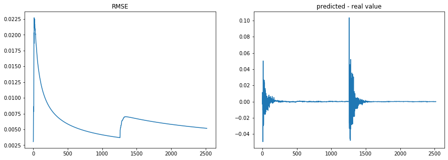
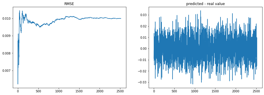
I wrote quickly this simple example to showcase Creme; an online linear regression on noisy time series containing a breakpoint:
%matplotlib inline
import matplotlib.pyplot as plt
import numpy as np
from numpy.random import normal
from creme import compose
from creme import linear_model
from creme import metrics
from creme import preprocessing
nb_years = 10
nb_days = nb_years * 252
break_nb_days = int(nb_years / 2 * 252)
X = [{'feature1': normal(scale=0.01),
'feature2': normal(scale=0.01),
'feature3': normal(scale=0.01),} for i in range(nb_days)]
signal = [(x,
0.8 * x['feature1'] + 0.6 * x['feature2'] - 2.3 * x['feature3']
if i < break_nb_days else
-2.3 * x['feature1'] + 0.6 * x['feature2'] + 0.8 * x['feature3'])
for i, x in enumerate(X)]
noise = [(x,
normal(scale=0.01))
for x in X]
def mix_signal_noise(signal, noise, alpha=0.5):
vol_noise = np.std([y for x, y in noise])
vol_signal = np.std([y for x, y in signal])
return [(x,
alpha * y_signal +
(1 - alpha) * (vol_signal / vol_noise) * y_noise)
for ((x, y_signal), (_, y_noise)) in zip(signal, noise)]
def apply_regression(data):
model = compose.Pipeline(
preprocessing.StandardScaler(),
linear_model.LinearRegression()
)
metric = metrics.RMSE()
preds = []
reals = []
rmses = []
for x, y in data:
y_pred = model.predict_one(x)
metric = metric.update(y, y_pred)
model = model.fit_one(x, y)
rmses.append(metric.get())
preds.append(y_pred)
reals.append(y)
plt.figure(figsize=(15, 5))
plt.subplot(1, 2, 1)
plt.plot(rmses)
plt.title('RMSE')
plt.subplot(1, 2, 2)
plt.plot([p - r for (p, r) in zip(preds, reals)])
plt.title('predicted - real value')
plt.show()
apply_regression(signal)
apply_regression(noise)
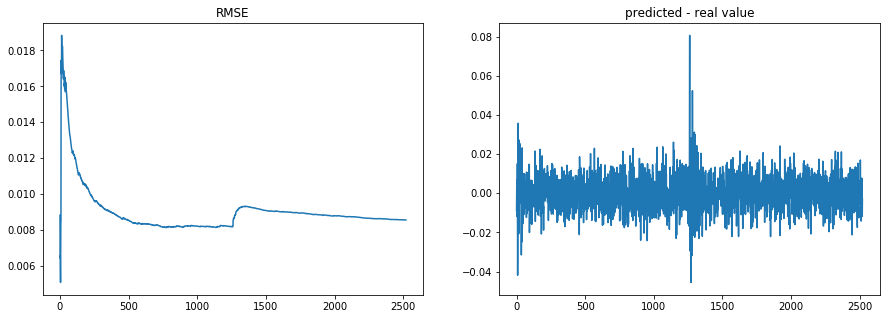
X_y = mix_signal_noise(signal, noise, alpha=0.7)
apply_regression(X_y)
Eason Suen - Deep Reinforcement Learning – A Quick Dive
Eason presented a broad picture of the current state of Reinforcement Learning, several branches: Q-learning, policy gradients, actor critic, evolution strategy, model-based RL. For each approach, he described the pros and cons, and how they relate to each other.
Several pointers are listed, an entertaining video to watch is the Multi-Agent Hide and Seek from OpenAI. Their gym is a good place to start learning. Google Research Football or AWS DeepRacer are other interesting projects to learn while having fun.
As expected in Hong Kong, many questions about the applications of such technology in Finance to learn how to trade markets. Eason take-on: Trading markets may not be where Reinfocement Learning shines the most as the typical use case for Reinforcement Learning are problems where the decision process is complex but the prediction part is easy (e.g. a computer vision problem), whereas in trading markets the decision process is rather simple (buy low sell high) compared to the prediction part which is close to impossible.