How to define an intrisic Mean of Correlation Matrices in a Riemannian sense?
How to define an intrisic Mean of Correlation Matrices in a Riemannian sense?
In this blog post, only questions, no answers.
The Riemannian geometry of the PSD cone (the set of covariance matrices) is rather well understood (for example, these slides or these slides for an overview of some mathematical properties). The inner product usually considered (depending smoothly on point $\Sigma$) is $<P_1, P_2>_\Sigma = Trace(\Sigma^{-1} P_1 \Sigma^{-1} P_2)$.
Besides enjoying many invariance properties, this Riemannian metric has the compelling property that its associated distance is equal to twice the Fisher-Rao distance, a Riemannian metric on the space of Gaussian probability densities $\mathcal{N}(0, \Sigma)$.
This connection between these two Riemannian metrics on very similar spaces (Gaussian distributions whose densities are parameterized with the same mean and a covariance can be identified to the covariance matrices) brings up a nice statistical interpretation via the Fréchet–Darmois–Cramér–Rao inequality:
The curvature of the covariance matrices space induced by the Riemannian metric is a simple function of the statistical estimation uncertainty.
Indeed, the Fréchet–Darmois–Cramér–Rao inequality essentially says that for an unbiased estimator, its variance is lower bounded by the reciprocal of the Fisher information (the Fisher-Rao Riemannian metric is a quadratic form of the Fisher information matrix): The higher the Fisher information, the lower the variance (and conversely). That means, for values that are hard to estimate (high variance) the space is rather flat whereas for values that are easy to estimate (low variance) the space is more curved.
To illustrate more precisely this idea, let’s consider the following small example: Bivariate centered Gaussian distributions whose densities are parameterized by 2 x 2 correlation matrices.
Let’s first derive the Fisher information:
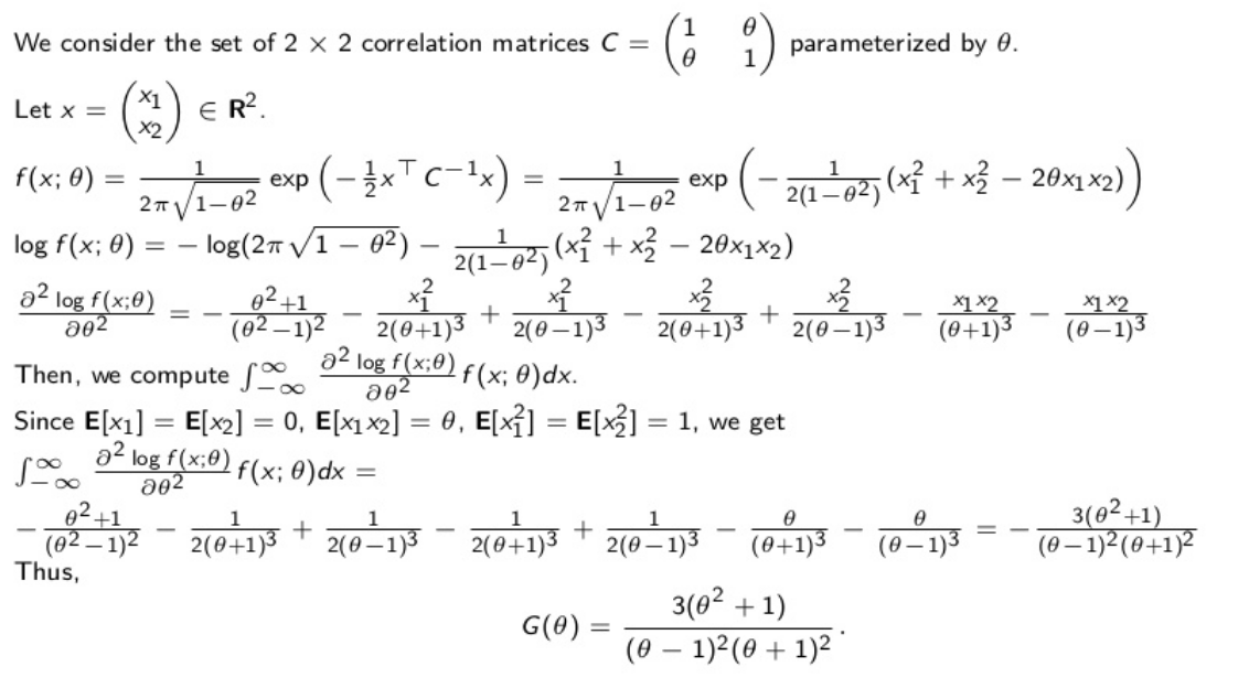
From the Fisher information $G(\rho)$, we can obtain the Fréchet–Darmois–Cramér–Rao lower bound for the variance of the correlation estimator:
We display the values below. Higher absolute correlation, lower lower bound for the estimator variance.
import operator
import numpy as np
from scipy.linalg import sqrtm
from scipy.linalg import fractional_matrix_power
from numpy.linalg import inv, eig
from matplotlib import pyplot as plt
from matplotlib import animation
from mpl_toolkits.mplot3d import Axes3D
from matplotlib import cm
from pprint import pprint


def fisher_information(rho):
    return ((rho - 1)**2 * (rho + 1)**2) / (3 * (rho**2 + 1))

rhos = np.linspace(-1, 1, 1000)
plt.plot(rhos, [fisher_information(rho) for rho in rhos])
plt.title(r'$var(\widehat{\rho}) \geq ' +
          r'\dfrac{(\rho - 1)^2(\rho + 1)^2}{3(\rho^2 + 1)}$',
          fontsize=16)
plt.show()
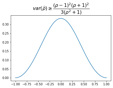
Remark: The uncertainty is very high when estimating correlations of low (absolute) values: $\sqrt{0.30} \approx 0.55$. Pretty big standard deviation for a coefficient taking values in $[-1,1]$!
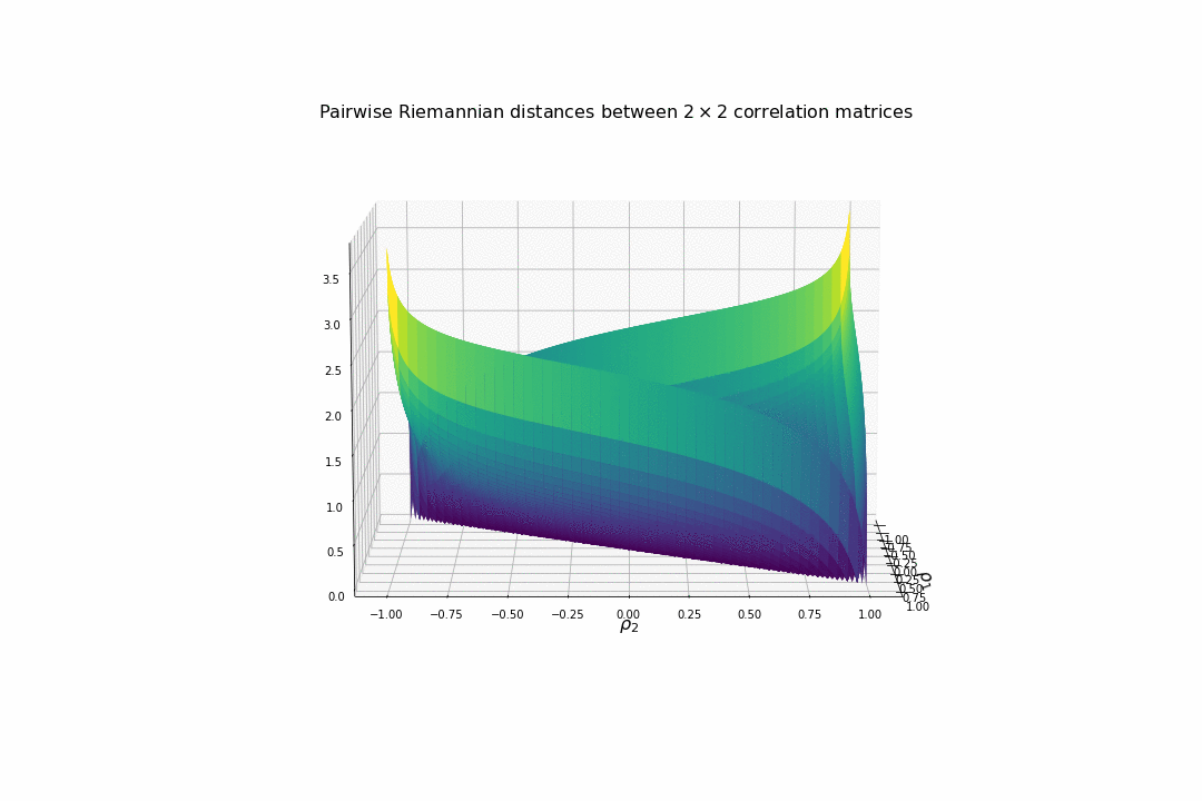
Now, we visualize what it means in terms of distances between two correlation matrices.
We display below the surface of all the pairwise distances between any two correlation matrices.
# Riemannian distance(A, B) = (sum_i ln(lambda_i)^2)^(1/2),
# where lambda_i are the A^(-1) * B
def riemann_dist(A, B):
    eigenvals, eigenvecs = eig(inv(A).dot(B))
    return np.sqrt(np.sum(np.log(eigenvals)**2))

N = 500
Z = np.zeros((N, N))
for i, rho_1 in enumerate(np.linspace(-0.99, 0.99, N)):
    corr_1 = np.array([[1, rho_1],
                       [rho_1, 1]])
    for j, rho_2 in enumerate(np.linspace(-0.99, 0.99, N)):
        corr_2 = np.array([[1, rho_2],
                           [rho_2, 1]])

        dist = 0.5 * riemann_dist(corr_1, corr_2)
        Z[i, j] = dist

X = np.outer(np.linspace(-0.99, 0.99, N), np.ones(N))
Y = X.copy().T

fig = plt.figure(figsize=(15, 10))
ax = plt.axes(projection='3d')

ax.plot_surface(X, Y, Z, rcount=100, ccount=100,
                cmap='viridis', edgecolor='none',
                linewidth=0, antialiased=True, alpha=0.9)
ax.set_title(r'Pairwise Riemannian distances between ' +
             r'$2 \times 2$ correlation matrices' + "\n",
             fontsize=16)
plt.xlabel(r'$\rho_1$', fontsize=16)
plt.ylabel(r'$\rho_2$', fontsize=16)
plt.show()
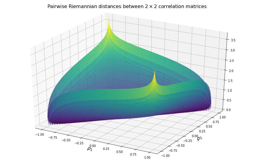
For high (absolute) correlation values, a small change of $d\rho$ in the correlation value yields to a relatively big change in distance in comparison to the same small change applied to low (absolute) correlation values. The space is more curved at the high (absolute) correlation values.
We understand why this Riemannian metric is prefered by statisticians: The space curvature allows for a better discrimination between signal and noise (due to statistical estimation) compared to a flat (say Euclidean, or Wasserstein) space.
def init():
    ax.plot_surface(X, Y, Z, rcount=50, ccount=50,
                    cmap='viridis', edgecolor='none')
    return fig,

def animate(i):
    ax.view_init(elev=10, azim=i*4)
    return fig,

anim = animation.FuncAnimation(
    fig, animate, init_func=init, frames=90, interval=50,
    blit=True)

fn = 'pairwise_corr_dists'
anim.save(fn + '.mp4', writer='ffmpeg', fps=1000 / 50)
anim.save(fn + '.gif', writer='imagemagick', fps=1000 / 50)
plt.rcParams['animation.html'] = 'html5'
anim
After this short digression that motivated the use of a Riemannian metric and discussed its statistical interpretation, back to the initial question: How to define an intrisic Riemannian mean of correlation matrices?
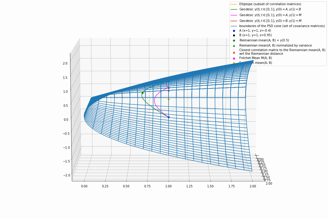
I read several Electrical Engineering papers which, when working with correlation matrices (this set is sometimes called an elliptope), use the fact that they are a subset of covariances matrices (this set is also called the Positive Semi Definite (PSD) cone), and then leverage the geometry of the PSD cone and its Riemannian metric $(S, g)$ to derive means, medians, and other geometric quantities from the correlation matrices.
However, it’s not clear to me this approach is valid. I will illustrate below, in the 2-dimensional case, why I think it is not necessarily the best way of doing it. For mathematicians, this can be expressed concisely:
The submanifold of correlation matrices $(E, g_E)$, with $g_E$ the Riemannian metric induced by $g$, is not a totally geodesic submanifold, i.e. a geodesic in $(E, g_E)$ is not necessarily a geodesic in $(S, g)$.
This can be easily seen in the animation below:
For PSD matrices of shape $2 \times 2$, the correlation matrices (elliptope) are restricted to a simple segment (x=1, y=1, z=-1..1) (displayed in orange).
Let’s consider $A$ and $B$ two correlation matrices. The geodesic between $A$ and $B$ when restrained to the elliptope (orange segment) is the sub-segment between $A$ and $B$.
However, the geodesic between $A$ and $B$ when considering $A$ and $B$ as points in $(S, g)$, i.e. covariance matrices, is the green curve.
Hence, $(E, g_E)$ is not totally geodesic.
Concerning the mean. The Riemannian mean of the two correlation matrices is the mid-point of the geodesic $\gamma(t=0.5)$ (or $=argmin_{\Sigma \in S} \sum_{i=1}^N d^2(\Sigma, \Sigma_i)$, where $d$ is the Riemannian distance, the general Fréchet mean definition for computing mean of more than two points) and displayed as a green dot below. The mean of two correlation matrices is not a correlation matrix, but a covariance matrix in general.
What should we do if we want or need to work only with correlation matrices?
-
Papers usually normalize the mean covariance $\Sigma$ by its variance to obtain the mean correlation $C$, that is $C = diag(\Sigma)^{-1/2} \Sigma diag(\Sigma)^{-1/2}$, displayed by a green triangle below.
-
A more geometrical way to project the mean covariance to the correlation space would be to find the nearest correlation matrix with respect to the Riemannian distance $d$ to this mean covariance, i.e. , where here $C_1 = A$ and $C_2 = B$. This closest correlation matrix is pictured as a red triangle below.
-
Searching for the correlation matrix solution of . It is displayed as a magenta dot below, with the geodesics from this point to $A$ (magenta), and to $B$ (red).
I believe 2. and 3. are equivalent. Proof?
Notice that, in general, approaches 1. and 2. (or 3.) do not yield the same “mean” correlation matrix.
Questions:
- So, what really should be the ‘Riemannian’ mean correlation matrix? I tend to prefer 2. or 3.
- Does one definition give better properties?
- What are these properties?
- Can we define an intrisic Riemannian mean with geodesic staying in the elliptope? (Not the case for 3.)
The animation below illustrates well the questionings:
def init():
    ax.plot_wireframe(X, Y, Z, ccount=20, rcount=20,
                      label='boundaries of the PSD cone ' +
                      '(set of covariance matrices)')
    return fig,

fig = plt.figure(figsize=(15, 10))
ax = Axes3D(fig)

# SPD cone
x = np.linspace(0, 2, num=500)
y = np.linspace(0, 2, num=500)
X, Y = np.meshgrid(x, y)
Z = np.sqrt(X * Y)

ax.plot_wireframe(X, Y, Z, ccount=20, rcount=20,
                  label='boundaries of the PSD cone ' +
                  '(set of covariance matrices)')
ax.plot_wireframe(X, Y, -Z, ccount=20, rcount=20)

# Elliptope
zline = np.linspace(-1, 1, 1000)
xline = [1] * len(zline)
yline = [1] * len(zline)

ax.plot3D(xline, yline, zline, 'orange',
          label='Elliptope (subset of correlation matrices)')


A = np.array([[1, -0.4],
              [-0.4, 1]])

B = np.array([[1, 0.95],
              [0.95, 1]])
ax.scatter(A[0,0],
           A[1,1],
           A[0,1],
           c='b', marker='o', s=30,
           label='A (x=1, y=1, z=-0.4)')
ax.scatter(B[0,0],
           B[1,1],
           B[0,1],
           c='k', marker='o', s=30,
           label='B (x=1, y=1, z=0.95)')


# Geodesic between A and B
# p(t) = A^(1/2) * (A^(-1/2) * B * A^(-1/2))^t * A^(1/2)
sqrt_A = fractional_matrix_power(A, 0.5)
inv_sqrt_A = fractional_matrix_power(A, -0.5)

x_geod = []
y_geod = []
z_geod = []
for t in np.linspace(0, 1, 100):
    geod_point = (
        sqrt_A.dot(fractional_matrix_power(
            inv_sqrt_A.dot(B.dot(inv_sqrt_A)), t)
                   .dot(sqrt_A)))
    x_geod.append(geod_point[0, 0])
    y_geod.append(geod_point[1, 1])
    z_geod.append(geod_point[0, 1])

ax.plot3D(x_geod, y_geod, z_geod, 'green',
          label=r'Geodesic $\gamma(t), t \in [0, 1],' +
          '\gamma(0) = A, \gamma(1) = B$')

# Riemannian mean
# the mean of two correlation matrix is not a correlation matrix in general
t = 0.5

riemann_mean = (sqrt_A.dot(fractional_matrix_power(
    inv_sqrt_A.dot(B.dot(inv_sqrt_A)), t).dot(sqrt_A)))

ax.scatter(riemann_mean[0,0],
           riemann_mean[1,1],
           riemann_mean[0,1],
           c='g', marker='o', s=30,
           label=r'Riemannian mean(A, B) = $\gamma(0.5)$')


# Riemannian mean, which is a covariance,
# "projected" back to the correlation space
# diag(Sigma)^(-1/2) * Sigma * diag(Sigma)^(-1/2)
corr_cvt = np.diag(np.sqrt(np.diag(riemann_mean)**(-1))).dot(
    riemann_mean.dot(
        np.diag(np.sqrt(np.diag(riemann_mean)**(-1)))))

ax.scatter(corr_cvt[0,0],
           corr_cvt[1,1],
           corr_cvt[0,1],
           c='g', marker='^', s=30,
           label='Riemannian mean(A, B) normalized by variance')


# point in the correlation space which minimizes the distance
# (in the Riemannian metric sense for the SPD space) to the covariance mean
closest_corr = min([(riemann_dist(np.array([[1, t], [t, 1]]),
                                  riemann_mean), np.array([[1, t], [t, 1]]))
                    for t in np.linspace(-0.99, 0.99, 5000)],
                   key=operator.itemgetter(0))[1]

ax.scatter(closest_corr[0,0],
           closest_corr[1,1],
           closest_corr[0,1],
           c='r', marker='^', s=30,
           label='Closest correlation matrix to the Riemannian mean(A, B)'
           + '\n' +  'wrt the Riemannian distance')

# Fréchet Mean:
# m = argmin_{C \in E} \sum_{i=1}^N d^2(C, C_i).
frechet_mean = min(
    [(riemann_dist(np.array([[1, t], [t, 1]]), A)**2 +
      riemann_dist(np.array([[1, t], [t, 1]]), B)**2,
      np.array([[1, t], [t, 1]]))
     for t in np.linspace(-0.99, 0.99, 5000)],
    key=operator.itemgetter(0))[1]

ax.scatter(frechet_mean[0,0],
           frechet_mean[1,1],
           frechet_mean[0,1],
           c='magenta', marker='o', s=30,
           label='Fréchet Mean M(A, B)')

# Geodesic between A and Frechet Mean M
# p(t) = A^(1/2) * (A^(-1/2) * M * A^(-1/2))^t * A^(1/2)
sqrt_A = fractional_matrix_power(A, 0.5)
inv_sqrt_A = fractional_matrix_power(A, -0.5)

x_geod = []
y_geod = []
z_geod = []
for t in np.linspace(0, 1, 100):
    geod_point = (
        sqrt_A.dot(fractional_matrix_power(
            inv_sqrt_A.dot(frechet_mean.dot(inv_sqrt_A)), t)
                   .dot(sqrt_A)))
    x_geod.append(geod_point[0, 0])
    y_geod.append(geod_point[1, 1])
    z_geod.append(geod_point[0, 1])

ax.plot3D(x_geod, y_geod, z_geod, 'magenta',
          label=r'Geodesic $\gamma(t), t \in [0, 1],' +
          '\gamma(0) = A, \gamma(1) = M$')

# Geodesic between B and Frechet Mean M
# p(t) = B^(1/2) * (B^(-1/2) * M * B^(-1/2))^t * B^(1/2)
sqrt_A = fractional_matrix_power(B, 0.5)
inv_sqrt_A = fractional_matrix_power(B, -0.5)

x_geod = []
y_geod = []
z_geod = []
for t in np.linspace(0, 1, 100):
    geod_point = (
        sqrt_A.dot(fractional_matrix_power(
            inv_sqrt_A.dot(frechet_mean.dot(inv_sqrt_A)), t)
                   .dot(sqrt_A)))
    x_geod.append(geod_point[0, 0])
    y_geod.append(geod_point[1, 1])
    z_geod.append(geod_point[0, 1])

ax.plot3D(x_geod, y_geod, z_geod, 'red',
          label=r'Geodesic $\gamma(t), t \in [0, 1],' +
          '\gamma(0) = B, \gamma(1) = M$')


# Euclidean mean
eucl_mean = (A + B) / 2

ax.scatter(eucl_mean[0,0],
           eucl_mean[1,1],
           eucl_mean[0,1],
           c='orange', marker='o', s=30,
           label='Euclidean mean(A, B)')


ax.legend()


anim = animation.FuncAnimation(
    fig, animate, init_func=init, frames=90, interval=50,
    blit=True)

fn = 'SPD_cone'
anim.save(fn + '.mp4', writer='ffmpeg', fps=1000 / 50)
anim.save(fn + '.gif', writer='imagemagick', fps=1000 / 50)
plt.rcParams['animation.html'] = 'html5'
anim