[Clustering] How and Where should you cut a dendrogram?
Introduction: Dendrogram cut-offs
Hierarchical clustering methods produce dendrograms which contain more information than mere flat clustering, for instance cluster proximity. A particular hierarchical clustering method, namely Single-Linkage, enjoys several nice theoretical properties (Zadeh and Ben-David, 2009) and (Carlsson and Mémoli, 2010) despite being known to give poor results in practice. Nonetheless, in (Awasthi et al., 2012), authors show that if the center-based clustering instance verifies some perturbation resilient properties, finding the optimal center-based clustering is possible in polynomial time by cutting efficiently the Single-Linkage dendrogram while in the general case, finding the optimal clustering is NP-hard.
The common practice to flatten dendrograms in $k$ clusters is to cut them off at constant height $k-1$. Yet it leads to poorer clusters than efficiently pruning the tree.
Dynamic Programming on dendrograms
A good intuition to have about optimization on trees is that it can usually be done in polynomial time using dynamic programming. Here, the approach has some theoretical ground since it has been shown that pruning the dendrogram produced by Single-Linkage using dynamic programming allows to recover in some well-defined cases the optimal clustering of a center-based clustering in polynomial time instead of the exponential time required in general case.
I think that, even in the general case, when one wants to extract a flat clustering from a dendrogram, it is worth applying a dynamic programming pruning: it allows to combine advantages of a hierarchical clustering and a center-based clustering.
Let $f$ be an objective function for evaluating the score of a partition. For benefiting from the theoretical properties, this one must be center-based and separable, cf. (Awasthi et al., 2012) for definitions. Here, we consider for $f$ the $k$-means objective function which is indeed a separable, center-based clustering objective.
We aim at computing
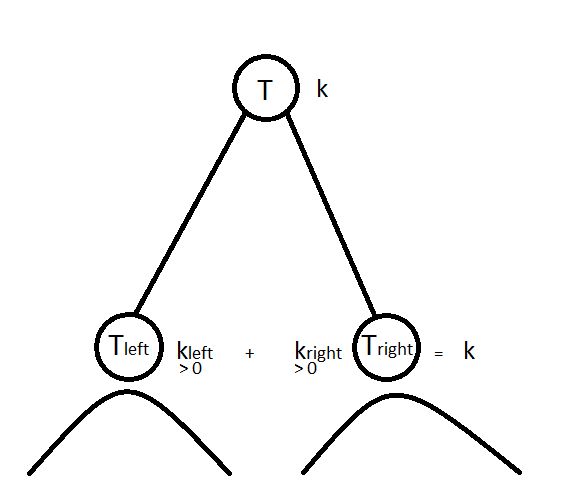
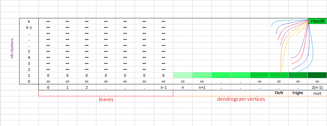
where $T$ is a dendrogram, $T_l$ and $T_r$ are respectively the left and right subtrees, and $k$ is the number of cluster we want to extract from $T$ to obtain a flat clustering from the hierarchical clustering described by $T$. Solving this optimization problem can be done in $O(k \cdot n\log n)$ time with dynamic programming. The basic idea is simple: we have to split data in $k$ clusters at the current node in $T$; if $k=1$ then all children of the current node are in the same cluster, if $k > 1$, then we can choose how to allocate the $k$ remaining clusters in the left and right subtrees; we split data points concerned by the left subtree $T_l$ in $k_l$ clusters and data points concerned by the right subtree $T_r$ in $k_r$ clusters such that we allocate all remaining clusters, i.e. $k_l + k_r = k$, and allocate at least one cluster in each subtree, i.e. $k_l, k_r > 0$; the best allocation is retained.
The $\text{compute_dyncut}$ function below solves this problem in a bottom-up fashion:
def compute_dyncut(data,nbClusters,children_map):
    nbVertices = max(children_map)
    inf = float("inf")
    dp = np.zeros((nbClusters+1,nbVertices+1)) + inf
    lcut = np.zeros((nbClusters+1,nbVertices+1))

    for i in range(0,dp.shape[1]):
        dp[1,i] = compute_intra_variance(i,children_map,data)

    root = max(children_map)
    for vertex in range(len(data),root+1):
        left_child, right_child = children_map[vertex]
        for k in range(2,nbClusters+1):
            vmin = inf
            kl_min = -1
            for kl in range(1,k):
                v = dp[kl,left_child] + dp[k-kl,right_child]
                if v < vmin:
                    vmin = v
                    kl_min = kl

            dp[k,vertex] = vmin
            lcut[k,vertex] = kl_min

    return dp,lcut
We illustrate the gain with respect to $f$ using the DP cut-off vs the constant height cut-off thanks to the $\text{bench_methods}$ function below:
Before benchmarking the `dyncut’ method, we define some ‘utils’ functions:
def build_dict_tree(linkage_matrix):
    tree = {}
    n = linkage_matrix.shape[0]+1
    for i in range(0,n-1):
        tree[linkage_matrix[i,0]] = n+i
        tree[linkage_matrix[i,1]] = n+i
    return tree

def build_children_map(tree):
    children_map = {}
    for k, v in tree.items():
        children_map[v] = children_map.get(v, [])
        children_map[v].append(int(k))
    return children_map

def build_children(vertex,children_map):
    children = []
    if vertex in children_map:
        left_child, right_child = children_map[vertex]
        if left_child in children_map:
            children.extend(build_children(left_child,children_map))
        else:
            children.extend([left_child])

        if right_child in children_map:
            children.extend(build_children(right_child,children_map))
        else:
            children.extend([right_child])

    return children

def get_var(data,subpop):
    intravar = 0
    center = np.mean(data[subpop],axis=0)
    for elem in subpop:
        x = data[elem] - center
        intravar += np.dot(x,x)
    return intravar

def compute_intra_variance(vertex,children_map,data):
    children = build_children(vertex,children_map)
    intravar = 0
    if children:
        intravar = get_var(data,children)

    return intravar

def compute_centers(data,target):
    centers = []
    for i in set(target):
        id_pts = [index for index,value in enumerate(target) if value == i]
        centers.append(np.mean(data[id_pts],axis=0))

    return centers

def compute_flat_dyn_clusters(cur_vertex,k,lcut,children_map):
    clusters = []
    #leaf
    if k == 1 and not cur_vertex in children_map:
        clusters.append([cur_vertex])
    #one cluster left, get the leaves
    if k == 1 and cur_vertex in children_map:
        leaves = build_children(cur_vertex,children_map)
        clusters.append(leaves)
    #recurse in left and right subtrees
    if k > 1:
        if cur_vertex in children_map:
            left_child,right_child = children_map[cur_vertex]
            clusters.extend(compute_flat_dyn_clusters(left_child,int(lcut[k,cur_vertex]),lcut,children_map))
            clusters.extend(compute_flat_dyn_clusters(right_child,int(k-lcut[k,cur_vertex]),lcut,children_map))

    return clusters

def compute_flat_cut_clusters(nbClusters,linkage_matrix):
    flat = fcluster(linkage_matrix,nbClusters,'maxclust')
    flat_clusters = []
    for i in range(1,len(set(flat))+1):
        flat_clusters.append( [index for index,value in enumerate(flat) if value == i] )

    return flat_clusters
And we load the ``Hello World!’’ of statistics: the Iris dataset.
from sklearn import datasets
iris = datasets.load_iris()
X = iris.data
Y = iris.target
Now, we can benchmark:
def bench_methods(data,nbClusters,methods):
    d = pdist(data)
    for method in methods:
        if method in ['centroid','ward','median']:
            linkage_matrix = linkage(data,method)
        else:
            linkage_matrix = linkage(d,method)
        tree = build_dict_tree(linkage_matrix)
        children_map = build_children_map(tree)
        dp,lcut = compute_dyncut(data,nbClusters,children_map)
        flat_dyn_clusters = compute_flat_dyn_clusters(max(children_map),nbClusters,lcut,children_map)
        flat_cut_clusters = compute_flat_cut_clusters(nbClusters,linkage_matrix)

        tot_dyn = 0
        tot_cut = 0
        for i in range(0,nbClusters):
            tot_dyn += get_var(data,flat_dyn_clusters[i])
            tot_cut += get_var(data,flat_cut_clusters[i])

        print("method:",method)
        print("intra-variance:", "(DP)",tot_dyn,"\t(cst height)",tot_cut)
        print("\n")
import numpy as np
from scipy.spatial.distance import pdist, squareform
from scipy.cluster.hierarchy import linkage, dendrogram, fcluster

nbClusters = 20
methods = ['single','complete','average','weighted','centroid','median','ward']

bench_methods(iris.data,nbClusters,methods)
method: single
intra-variance: (DP) 38.4374512821 	(cst height) 46.2485205803


method: complete
intra-variance: (DP) 15.5002502089 	(cst height) 15.5002502089


method: average
intra-variance: (DP) 15.9479145299 	(cst height) 18.4471483254


method: weighted
intra-variance: (DP) 15.9755833333 	(cst height) 17.0310744048


method: centroid
intra-variance: (DP) 16.8013257576 	(cst height) 22.1164536341


method: median
intra-variance: (DP) 17.5263907828 	(cst height) 19.1726534091


method: ward
intra-variance: (DP) 15.0222202381 	(cst height) 15.0222202381
We notice that DynCut finds clusters of lesser variance than those extracted at constant height cut in general.
Bonus: A sufficient condition for optimal clustering in polynomial time
According to (Awasthi et al., 2012), the $\alpha$-center proximity property, i.e. $\forall p \in S$, $c_i$ its nearest center, $\forall c_j \neq c_i$, $d(p,c_j) > \alpha d(p,c_i)$, with $\alpha \geq 2+\sqrt{3}$, is a sufficient condition to have min-stability, i.e. for any strict subset of some cluster the closest point to this subset not being part of it comes from this cluster, a necessary and sufficient condition for the Single-Linkage algorithm to produce a tree on clusters such that the optimal clustering forms a pruning of this tree.
def center_proximity(alpha,pt,centers):
    dists = []
    for center in centers:
        dists.append(np.linalg.norm(pt-center))
    minDist = min(dists)
    argmin = np.argmin(dists)
    for i in range(0,len(dists)):
        if not i == argmin:
            if dists[i] <= alpha*minDist:
                return False
    return True

def prop_viol_center_proximity(alpha,data,target):
    nb_viol = 0
    centers = compute_centers(data,target)
    for pt in data:
        if not center_proximity(alpha,pt,centers):
            nb_viol += 1
    return nb_viol / len(target)
def verif_center_proximity(alpha,data,target):
    return prop_viol_center_proximity(alpha,data,target) == 0
Notice that the iris dataset does not verify this condition: Indeed, this dataset is not linearly separable.
alpha = 2+np.sqrt(3)
verif_center_proximity(alpha,iris.data,iris.target)
False
More than half of the points in Iris data set violate the $\alpha$-center proximity property:
prop_viol_center_proximity(alpha,iris.data,iris.target)
0.5333333333333333
References
Awasthi P., Blum A., Sheffet O., 2012. Center-based Clustering under Perturbation Stability published in Information Processing Letters, Elsevier.
Carlsson G. and Mémoli F., 2010. Characterization, stability and convergence of hierarchical clustering methods published in The Journal of Machine Learning Research.
Zadeh R. B. and Ben-David S., 2009. A uniqueness theorem for clustering published in the Proceedings of the twenty-fifth conference on uncertainty in artificial intelligence.
Kleinberg J., 2003. An impossibility theorem for clustering published in Advances in neural information processing systems.
Meilă M., 2006. The uniqueness of a good optimum for k-means published in the Proceedings of the 23rd international conference on Machine learning, ACM.
Arthur D. and Vassilvitskii S., 2007. k-means++: The advantages of careful seeding published in the Proceedings of the eighteenth annual ACM-SIAM symposium on Discrete algorithms, Society for Industrial and Applied Mathematics.