[Clustering] How to sort a distance matrix
Following the Ecole Polytechnique - Data Science Summer School where I got several times questions about how I produced the sorted correlation matrices displayed in my poster, I decided to write this small blog post. Its goal is to illustrate how to sort a distance matrix so that eventual (hierarchical) clusters are blatant.
For illustration purpose, we will use the ‘Hello World!’ of datasets, the Iris dataset:
import numpy as np
from scipy.spatial.distance import pdist, squareform
from sklearn import datasets
from fastcluster import linkage

import matplotlib.pyplot as plt
%matplotlib inline
iris = datasets.load_iris()
iris.data.shape
(150, 4)
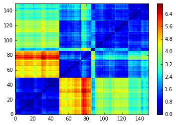
The dataset contains 150 points in R^4 (150 flowers described by 4 features). Using pdist we can compute a 150 x 150 distance matrix which is displayed below.
dist_mat = squareform(pdist(iris.data))

N = len(iris.data)
plt.pcolormesh(dist_mat)
plt.colorbar()
plt.xlim([0,N])
plt.ylim([0,N])
plt.show()
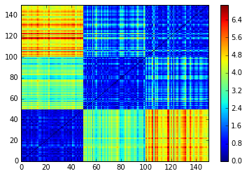
We can see that there is 3 noticeable clusters: one which is rather dense (bottom left) and far from the two others, and two which are quite close but differ in their respective distance to the (bottom left) third one.
These clusters correspond to the 3 classes that can be found in iris.target:
One which is linearly separable (the 0 class below, corresponding to the bottom left cluster in the distance matrix), and two which are not (classes 1 and 2, corresponding to the two rightmost clusters).
iris.target
array([0, 0, 0, 0, 0, 0, 0, 0, 0, 0, 0, 0, 0, 0, 0, 0, 0, 0, 0, 0, 0, 0, 0,
       0, 0, 0, 0, 0, 0, 0, 0, 0, 0, 0, 0, 0, 0, 0, 0, 0, 0, 0, 0, 0, 0, 0,
       0, 0, 0, 0, 1, 1, 1, 1, 1, 1, 1, 1, 1, 1, 1, 1, 1, 1, 1, 1, 1, 1, 1,
       1, 1, 1, 1, 1, 1, 1, 1, 1, 1, 1, 1, 1, 1, 1, 1, 1, 1, 1, 1, 1, 1, 1,
       1, 1, 1, 1, 1, 1, 1, 1, 2, 2, 2, 2, 2, 2, 2, 2, 2, 2, 2, 2, 2, 2, 2,
       2, 2, 2, 2, 2, 2, 2, 2, 2, 2, 2, 2, 2, 2, 2, 2, 2, 2, 2, 2, 2, 2, 2,
       2, 2, 2, 2, 2, 2, 2, 2, 2, 2, 2, 2])
Since the 150 data points are sorted according to their respective class, the clustering structure is already blatant.
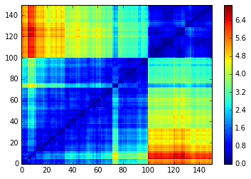
To showcase the usefulness of the proposed method for sorting dissimilarity matrices, we apply a random permutation to the data points. This is relevant as data points are usually provided in an arbitrary order and often without any labels.
X = iris.data[np.random.permutation(N),:]

dist_mat = squareform(pdist(X))

plt.pcolormesh(dist_mat)
plt.xlim([0,N])
plt.ylim([0,N])
plt.show()
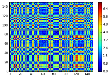
We can notice that is the general case, one cannot see any clustering structure on the raw distance matrix computed on the data points (which are provided in an arbitrary order).
The two functions allow us to sort dissimilarity matrices so that if there is a (hierarchical) clustering structure, one can see it on the distance matrix directly.
The process is in two steps essentially:
- compute a hierarchical tree (dendrogram) using an agglomerative hierarchical clustering algorithm
- traverse recursively the tree from top (root = all in the same cluster) to bottom (leaves = all points in their own singleton cluster); while traversing the tree, each branching helps to sort the points in a left vs. right subpart
At the end of the process all points are sorted according to order imposed by the dendrogram.
def seriation(Z,N,cur_index):
    '''
        input:
            - Z is a hierarchical tree (dendrogram)
            - N is the number of points given to the clustering process
            - cur_index is the position in the tree for the recursive traversal
        output:
            - order implied by the hierarchical tree Z

        seriation computes the order implied by a hierarchical tree (dendrogram)
    '''
    if cur_index < N:
        return [cur_index]
    else:
        left = int(Z[cur_index-N,0])
        right = int(Z[cur_index-N,1])
        return (seriation(Z,N,left) + seriation(Z,N,right))

def compute_serial_matrix(dist_mat,method="ward"):
    '''
        input:
            - dist_mat is a distance matrix
            - method = ["ward","single","average","complete"]
        output:
            - seriated_dist is the input dist_mat,
              but with re-ordered rows and columns
              according to the seriation, i.e. the
              order implied by the hierarchical tree
            - res_order is the order implied by
              the hierarhical tree
            - res_linkage is the hierarhical tree (dendrogram)

        compute_serial_matrix transforms a distance matrix into
        a sorted distance matrix according to the order implied
        by the hierarchical tree (dendrogram)
    '''
    N = len(dist_mat)
    flat_dist_mat = squareform(dist_mat)
    res_linkage = linkage(flat_dist_mat, method=method,preserve_input=True)
    res_order = seriation(res_linkage, N, N + N-2)
    seriated_dist = np.zeros((N,N))
    a,b = np.triu_indices(N,k=1)
    seriated_dist[a,b] = dist_mat[ [res_order[i] for i in a], [res_order[j] for j in b]]
    seriated_dist[b,a] = seriated_dist[a,b]

    return seriated_dist, res_order, res_linkage
Observe that the order obtained depends strongly on the agglomerative hierarchical clustering method chosen. In particular, using these 4 methods, we do not recover the original order (which was not supposed to be ‘optimal’ - whatever that means - intraclass-wise anyway).
methods = ["ward","single","average","complete"]
for method in methods:
    print("Method:\t",method)

    ordered_dist_mat, res_order, res_linkage = compute_serial_matrix(dist_mat,method)

    plt.pcolormesh(ordered_dist_mat)
    plt.xlim([0,N])
    plt.ylim([0,N])
    plt.show()
Method: ward
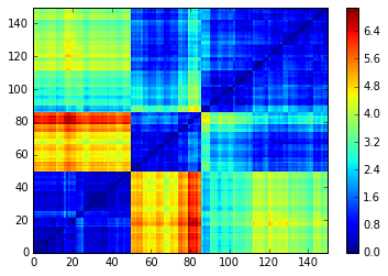
Method: single
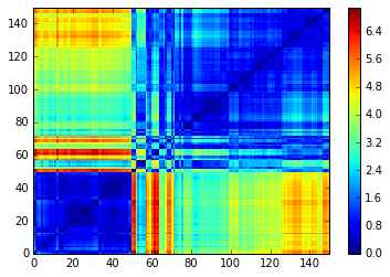
Method: average
Method: complete
To conclude, using a hierarchical clustering method in order to sort a distance matrix is a heuristic to find a good permutation among the n! (in this case, the 150! = 5.713384e+262) possible permutations. It won’t in general find the best permutation (whatever that means) as you do not choose the optimization criterion, but it is inherited from the clustering algorithm itself.
There are other techniques available, for example based on eigenvectors (cf. this paper for a survey of reordering algorithms for matrices).
Finally, one should prefer to visualize the sorted distance matrix using a hierarchical clustering algorithm if one intends to use the same hierarchical clustering algorithm for further processing: It helps to find the underlying number of clusters, to understand how ‘dense’ a cluster is (color/values of the block on the diagonal) or how ‘far’ it is from other clusters (color/values outside the diagonal). It can also help to spot spurious clusters, i.e. clusters that were built by the clustering algorithm but which are not ‘dense’ at all and sometimes also distant from everything else.