A Monte Carlo study of the ``Combination of Rankings'' methods
A Monte Carlo study of the ``Combination of Rankings’’ methods
In the previous blog post titled Combination of Rankings, we introduced a method to combine several rankings, each one weighted by some confidence, into a final one having greater predictive power (higher correlation with the true outcome, i.e. observed ranking). We explained there the motivation for using a network-based approach instead of the baseline average: dealing with widely heterogeneous coverage, missing data, and biases in the missing data. The network-based approach is supposed to outperform significantly the naive avearge one when there is a strong bias in the missing data. For example, the latent best ranks have usually data which are lacking for the latent lowest ranks. In that case, the worst of the best ranks in this partial ranking will end up having the lowest ranks possible, which produce a very negative contribution in the final average ranking. The network-based approach does not suffer from this problem.
In this blog post however, we will not assume that missing data have some coverage biases, i.e. we will sample uniformly (without replacement) the objects to rank, with a coverage between 2% and 50% (uniform sampling again) of the total number of objects. We will also sample uniformly the confidence (between 1% and 60%) associated to each ranking.
We are therefore only testing for the eventual benefit of using the network-based approach over the average one in the case of totally random missing data. That is, not the best case scenario.
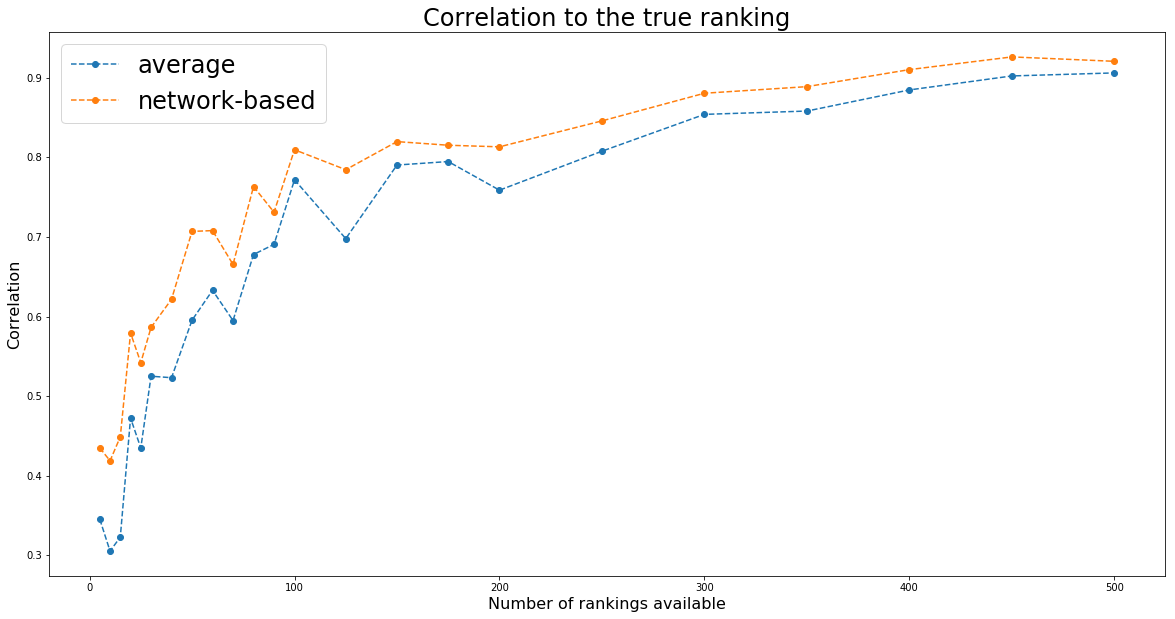
We will also vary the number of available rankings to check whether with a large number of rankings the two methods converge to the same outcome (which might be the case here as the missing data are totally random, thus no systematic error biases).
import pandas as pd
import numpy as np
import networkx as nx
from scipy.linalg import block_diag
import matplotlib.pyplot as plt
%matplotlib inline

np.random.seed(seed=42)
def build_graph(rankings):
    rank_graph = nx.DiGraph()
    for ranking, ic in rankings:
        for node in ranking.values():
            rank_graph.add_node(node)
    for ranking, ic in rankings:
        for rank_up in range(1, len(ranking)):
            for rank_dn in range(rank_up + 1, len(ranking) + 1):
                u = ranking[rank_up]
                v = ranking[rank_dn]

                if u in rank_graph and v in rank_graph[u]:
                    rank_graph.edges[u, v]['weight'] += ic
                else:
                    rank_graph.add_edge(u, v, weight=ic)

    return rank_graph
def build_markov_chain(rank_graph):
    for node in rank_graph.nodes():
        sum_weights = 0

        for adj_node in rank_graph[node]:
            sum_weights += rank_graph[node][adj_node]['weight']

        for adj_node in rank_graph[node]:
            rank_graph.edges[node, adj_node]['weight'] /= sum_weights

    return rank_graph
def random_walk(markov_chain, counts, max_random_steps=1000):
    cur_step = 0
    current_node = graph_nodes[np.random.randint(len(graph_nodes))]
    while cur_step < max_random_steps:
        counts[current_node] += 1
        neighbours = [(adj, markov_chain[current_node][adj]['weight'])
                      for adj in markov_chain[current_node]]

        adj_nodes = [adj for adj, w in neighbours]
        adj_weights = [w for adj, w in neighbours]

        if not adj_nodes:
            return counts

        current_node = np.random.choice(adj_nodes, p=adj_weights)

        cur_step += 1

    return counts
Let’s generate some artificial data. Let’s assume that our goal is to rank 250 assets according to their performance in 1 year (252 trading days). Basically, we will just sample random noise, and look at the ‘‘performance’’ of these 250 random walks. This ‘‘performance’’ ranking will be the true ranking that ‘‘experts’’ try to predict with more or less success on a subset of all the available assets. To generate the ‘‘experts’’ predictions, we will just sample time series correlated with the original sample. The correlation is in fact the confidence in the expert prediction. We have thus generated several rankings having some predictive power of the true ranking. We will combine them using both the network-based approach and the naive average one.
nb_assets = 250
nb_observations = 1 * 252
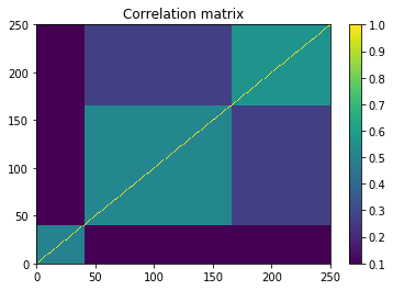
# useless sophistication to make the time series more ``realistic''
background_correlation = 0.3 * np.ones((nb_assets, nb_assets))
sector_1 = 0.6 * np.ones((nb_assets//6, nb_assets//6))
sector_2 = 0.75 * np.ones((nb_assets//2, nb_assets//2))
sector_3 = 0.9 * np.ones((int(nb_assets*(1 - 1/6 - 1/2) + 1),
int(nb_assets*(1 - 1/6 - 1/2) + 1)))
sector_background = 0.5 * np.ones((int(nb_assets*(1 - 1/6)) + 1,
int(nb_assets*(1 - 1/6)) + 1))
correl = (background_correlation +
block_diag(sector_1, sector_background) +
block_diag(sector_1, sector_2, sector_3)) / 3
np.fill_diagonal(correl, 1)
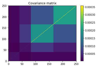
mean_returns = np.zeros(nb_assets)
volatilities = ([0.1 / np.sqrt(252)] * (nb_assets // 3) +
[0.3 / np.sqrt(252)] * (nb_assets - nb_assets // 3))
covar = np.multiply(correl,
np.outer(np.array(volatilities),
np.array(volatilities)))
plt.pcolormesh(correl)
plt.colorbar()
plt.title('Correlation matrix')
plt.show()

plt.pcolormesh(covar)
plt.colorbar()
plt.title('Covariance matrix')
plt.show()
residual_returns = np.random.multivariate_normal(
    mean_returns, cov=covar, size=nb_observations)

residual_returns = pd.DataFrame(residual_returns)
plt.figure(figsize=(20, 10))
plt.plot(100 + residual_returns.cumsum())
plt.show()
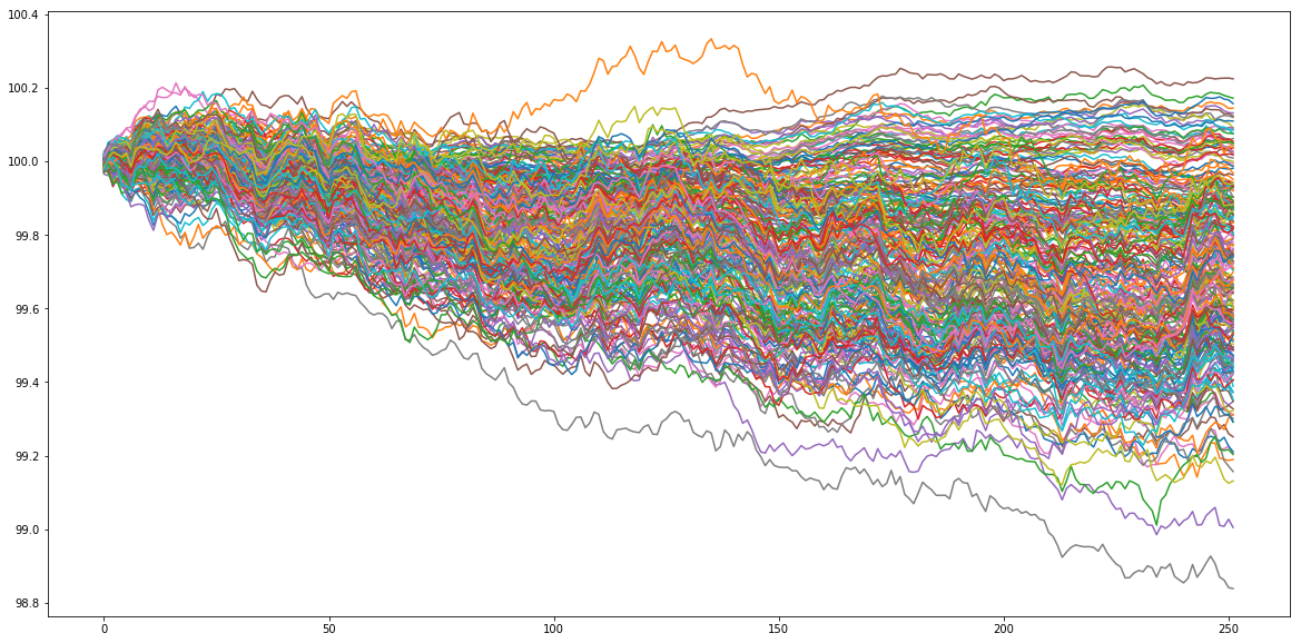
ranked_cumulative_residual_returns = (residual_returns
                                      .sum()
                                      .rank(ascending=False))
ranked_cumulative_residual_returns.head()
0    72.0
1     4.0
2     2.0
3    48.0
4     5.0
dtype: float64
We are now applying the two approaches for an increasing number of rankings available.
nb_experts_available = [
    5,
    10,
    15,
    20,
    25,
    30,
    40,
    50,
    60,
    70,
    80,
    90,
    100,
    125,
    150,
    175,
    200,
    250,
    300,
    350,
    400,
    450,
    500,
]
results = {}

for nb_experts in nb_experts_available:

    prediction_rankings = []

    for expert in range(nb_experts):
        confidence = np.random.randint(1, 61) / 100
        pct_coverage = np.random.randint(2, 51) / 100
        expert_coverage = np.random.choice(nb_assets, replace=False,
                                           size=int(nb_assets * pct_coverage))

        predictions = []
        for node in expert_coverage:
            prediction = (confidence * residual_returns[node] +
                          np.sqrt(1 - confidence**2) * np.random.normal(
                              0, np.std(residual_returns[node]), nb_observations))
            predictions.append(prediction)

        expert_predictions = pd.DataFrame(np.array(predictions).T,
                                          columns=expert_coverage)
        ranked_cumulated_predictions = (
            expert_predictions
            .sum()
            .rank(ascending=False))

        prediction_rankings.append(
            ({value: key for key, value in dict(ranked_cumulated_predictions).items()},
             confidence))

    rank_graph = build_graph(prediction_rankings)
    markov_chain = build_markov_chain(rank_graph)

    graph_nodes = list(markov_chain.nodes())

    max_random_steps = 10000
    counts = {node: 0 for node in graph_nodes}

    nb_jumps = 100
    for jump in range(nb_jumps):
        counts = random_walk(markov_chain, counts, max_random_steps)

    # true ranking
    true_ranking = sorted([(key, value)
                           for key, value in dict(ranked_cumulative_residual_returns).items()],
                          key=lambda x: x[1])
    true_ranking = pd.Series([count for node, count in true_ranking],
                         index=[node for node, count in true_ranking])

    # rank graph method
    final_ranking = sorted([(node, count) for node, count in counts.items()],
                           key=lambda x: x[0])

    graph_ranking = (pd.Series([count for node, count in final_ranking],
                              index=[node for node, count in final_ranking])
                     .rank(ascending=True))

    # average ranking
    rankings = pd.DataFrame(np.nan,
                            columns=sorted(graph_nodes),
                            index=range(len(prediction_rankings)))
    for idrank in range(len(prediction_rankings)):
        for rank, asset in prediction_rankings[idrank][0].items():
            rankings[asset].loc[idrank] = rank / len(prediction_rankings[idrank][0])

    sum_weights = sum([prediction_rankings[idrank][1]
                       for idrank in range(len(prediction_rankings))])
    average_rankings = (rankings
                        .multiply([prediction_rankings[idrank][1] / sum_weights
                                   for idrank in range(len(prediction_rankings))],
                                  axis='rows')
                        .sum(axis=0))

    average_ranking = average_rankings.rank(ascending=True)


    results[nb_experts] = {
        'avg': average_ranking.corr(true_ranking, method='spearman'),
        'graph': graph_ranking.corr(true_ranking, method='spearman'),
        'correl': average_ranking.corr(graph_ranking, method='spearman')}

    print(nb_experts)
    print(results[nb_experts])
5
{'avg': 0.3450563538272528, 'graph': 0.43474963173018455, 'correl': 0.8113000842678526}
10
{'avg': 0.30504783069150504, 'graph': 0.4185906517495598, 'correl': 0.7813370605773966}
15
{'avg': 0.3226158400557813, 'graph': 0.44871828717235357, 'correl': 0.8213010005388195}
20
{'avg': 0.4723310132962127, 'graph': 0.5791964167599003, 'correl': 0.9227381113070862}
25
{'avg': 0.43468558103381266, 'graph': 0.5419874904708406, 'correl': 0.886625856952652}
30
{'avg': 0.5249206547304757, 'graph': 0.5862288378853265, 'correl': 0.9375705371830438}
40
{'avg': 0.5230720491527865, 'graph': 0.6217038560976859, 'correl': 0.9445131709438144}
50
{'avg': 0.5953903902462439, 'graph': 0.7070315035044593, 'correl': 0.9593728867648482}
60
{'avg': 0.6329469591513464, 'graph': 0.7080225120025956, 'correl': 0.9532852147486358}
70
{'avg': 0.5949334229347669, 'graph': 0.6654963428182809, 'correl': 0.9290749571117007}
80
{'avg': 0.6779709115345846, 'graph': 0.7634083682793666, 'correl': 0.9405637989050101}
90
{'avg': 0.6906976431622905, 'graph': 0.7311778283900421, 'correl': 0.9548888435764108}
100
{'avg': 0.7718780780492487, 'graph': 0.8097096870700276, 'correl': 0.9675882956294934}
125
{'avg': 0.6979346229539671, 'graph': 0.7846239125178474, 'correl': 0.9478724399004538}
150
{'avg': 0.7904816397062352, 'graph': 0.8199252607844635, 'correl': 0.9692692910074586}
175
{'avg': 0.7948508616137858, 'graph': 0.8153705577876906, 'correl': 0.9723463363757362}
200
{'avg': 0.7588679498871982, 'graph': 0.8133665831973623, 'correl': 0.9625094225663696}
250
{'avg': 0.8078494695915135, 'graph': 0.8459663917192989, 'correl': 0.9724233138275763}
300
{'avg': 0.8541790428646857, 'graph': 0.8807571227467537, 'correl': 0.9758398416056108}
350
{'avg': 0.8583493495895934, 'graph': 0.8890416382352168, 'correl': 0.9764692193653824}
400
{'avg': 0.8849118225891613, 'graph': 0.9104630698814674, 'correl': 0.9805696432704211}
450
{'avg': 0.9024954639274227, 'graph': 0.9264329923039764, 'correl': 0.9793836503471612}
500
{'avg': 0.9063109489751837, 'graph': 0.9208994280805123, 'correl': 0.9815344637346255}
plt.figure(figsize=(20, 10))
plt.plot(nb_experts_available,
         [results[nb_experts]['avg'] for nb_experts in nb_experts_available],
         '--o', label='average')
plt.plot(nb_experts_available,
         [results[nb_experts]['graph'] for nb_experts in nb_experts_available],
         '--o', label='network-based')
plt.title('Correlation to the true ranking', fontsize=24)
plt.legend(fontsize=24)
plt.xlabel('Number of rankings available', fontsize=16)
plt.ylabel('Correlation', fontsize=16)
plt.show()