``Combination of Rankings'' - The Full Coverage Case
``Combination of Rankings’’ - The Full Coverage Case
We follow the same experimental setup as in the blog post A Monte Carlo study of the ``Combination of Rankings’’ methods, but here we will set the coverage at 100% for all the rankings to combine.
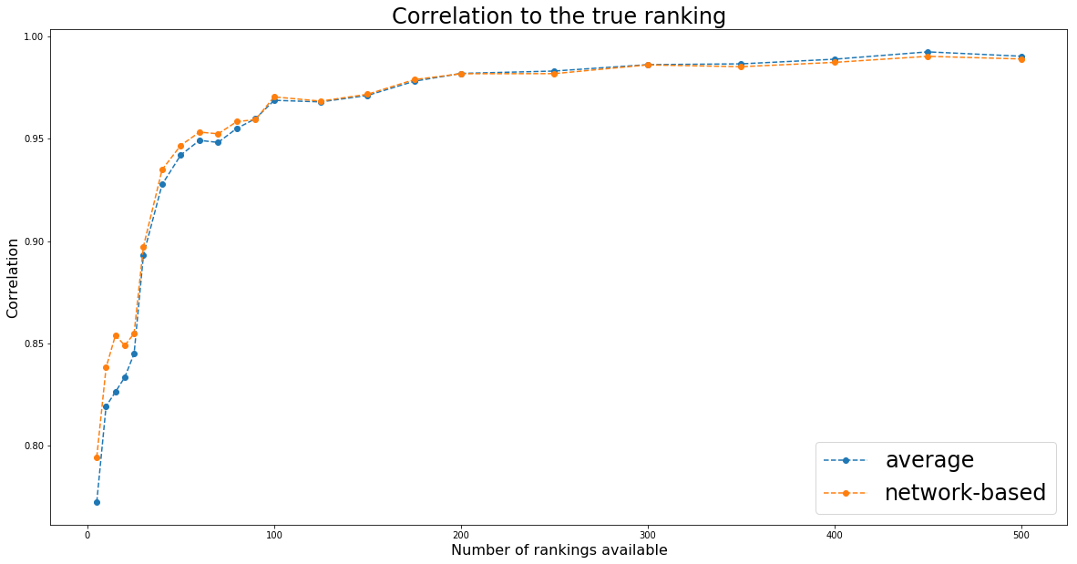
Question: How do the two methods (i.e. average and network-based) compare?
TL;DR Essentially the same.
import pandas as pd
import numpy as np
import networkx as nx
from scipy.linalg import block_diag
import matplotlib.pyplot as plt
%matplotlib inline

np.random.seed(seed=42)
def build_graph(rankings):
    rank_graph = nx.DiGraph()
    for ranking, ic in rankings:
        for node in ranking.values():
            rank_graph.add_node(node)
    for ranking, ic in rankings:
        for rank_up in range(1, len(ranking)):
            for rank_dn in range(rank_up + 1, len(ranking) + 1):
                u = ranking[rank_up]
                v = ranking[rank_dn]

                if u in rank_graph and v in rank_graph[u]:
                    rank_graph.edges[u, v]['weight'] += ic
                else:
                    rank_graph.add_edge(u, v, weight=ic)

    return rank_graph
def build_markov_chain(rank_graph):
    for node in rank_graph.nodes():
        sum_weights = 0

        for adj_node in rank_graph[node]:
            sum_weights += rank_graph[node][adj_node]['weight']

        for adj_node in rank_graph[node]:
            rank_graph.edges[node, adj_node]['weight'] /= sum_weights

    return rank_graph
def random_walk(markov_chain, counts, max_random_steps=1000):
    cur_step = 0
    current_node = graph_nodes[np.random.randint(len(graph_nodes))]
    while cur_step < max_random_steps:
        counts[current_node] += 1
        neighbours = [(adj, markov_chain[current_node][adj]['weight'])
                      for adj in markov_chain[current_node]]

        adj_nodes = [adj for adj, w in neighbours]
        adj_weights = [w for adj, w in neighbours]

        if not adj_nodes:
            return counts

        current_node = np.random.choice(adj_nodes, p=adj_weights)

        cur_step += 1

    return counts
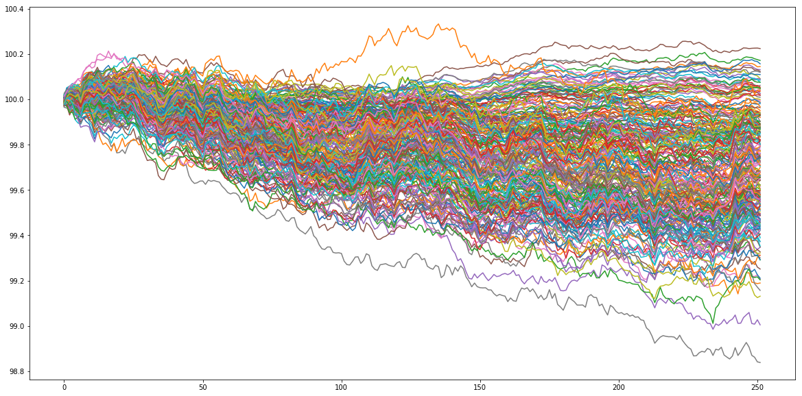
Let’s generate some artificial data. Let’s assume that our goal is to rank 250 assets according to their performance in 1 year (252 trading days). Basically, we will just sample random noise, and look at the ‘‘performance’’ of these 250 random walks. This ‘‘performance’’ ranking will be the true ranking that ‘‘experts’’ try to predict with more or less success on a subset of all the available assets. To generate the ‘‘experts’’ predictions, we will just sample time series correlated with the original sample. The correlation is in fact the confidence in the expert prediction. We have thus generated several rankings having some predictive power of the true ranking. We will combine them using both the network-based approach and the naive average one.
nb_assets = 250
nb_observations = 1 * 252

# useless sophistication to make the time series more ``realistic''
background_correlation = 0.3 * np.ones((nb_assets, nb_assets))
sector_1 = 0.6 * np.ones((nb_assets//6, nb_assets//6))
sector_2 = 0.75 * np.ones((nb_assets//2, nb_assets//2))
sector_3 = 0.9 * np.ones((int(nb_assets*(1 - 1/6 - 1/2) + 1),
                          int(nb_assets*(1 - 1/6 - 1/2) + 1)))
sector_background = 0.5 * np.ones((int(nb_assets*(1 - 1/6)) + 1,
                                   int(nb_assets*(1 - 1/6)) + 1))


correl = (background_correlation +
          block_diag(sector_1, sector_background) +
          block_diag(sector_1, sector_2, sector_3)) / 3
np.fill_diagonal(correl, 1)


mean_returns = np.zeros(nb_assets)
volatilities = ([0.1 / np.sqrt(252)] * (nb_assets // 3) +
                [0.3 / np.sqrt(252)] * (nb_assets - nb_assets // 3))
covar = np.multiply(correl,
                    np.outer(np.array(volatilities),
                             np.array(volatilities)))
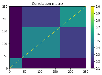
plt.pcolormesh(correl)
plt.colorbar()
plt.title('Correlation matrix')
plt.show()
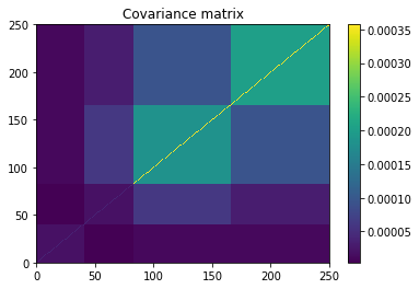
plt.pcolormesh(covar)
plt.colorbar()
plt.title('Covariance matrix')
plt.show()
residual_returns = np.random.multivariate_normal(
    mean_returns, cov=covar, size=nb_observations)

residual_returns = pd.DataFrame(residual_returns)
plt.figure(figsize=(20, 10))
plt.plot(100 + residual_returns.cumsum())
plt.show()
ranked_cumulative_residual_returns = (residual_returns
                                      .sum()
                                      .rank(ascending=False))
ranked_cumulative_residual_returns.head()
0    72.0
1     4.0
2     2.0
3    48.0
4     5.0
dtype: float64
We are now applying the two approaches for an increasing number of rankings available.
nb_experts_available = [
    5,
    10,
    15,
    20,
    25,
    30,
    40,
    50,
    60,
    70,
    80,
    90,
    100,
    125,
    150,
    175,
    200,
    250,
    300,
    350,
    400,
    450,
    500,
]
results = {}

for nb_experts in nb_experts_available:

    prediction_rankings = []

    for expert in range(nb_experts):
        confidence = np.random.randint(1, 61) / 100
        pct_coverage = 1
        expert_coverage = np.random.choice(nb_assets, replace=False,
                                           size=int(nb_assets * pct_coverage))

        predictions = []
        for node in expert_coverage:
            prediction = (confidence * residual_returns[node] +
                          np.sqrt(1 - confidence**2) * np.random.normal(
                              0, np.std(residual_returns[node]), nb_observations))
            predictions.append(prediction)

        expert_predictions = pd.DataFrame(np.array(predictions).T,
                                          columns=expert_coverage)
        ranked_cumulated_predictions = (
            expert_predictions
            .sum()
            .rank(ascending=False))

        prediction_rankings.append(
            ({value: key for key, value in dict(ranked_cumulated_predictions).items()},
             confidence))

    rank_graph = build_graph(prediction_rankings)
    markov_chain = build_markov_chain(rank_graph)

    graph_nodes = list(markov_chain.nodes())

    max_random_steps = 10000
    counts = {node: 0 for node in graph_nodes}

    nb_jumps = 200
    for jump in range(nb_jumps):
        counts = random_walk(markov_chain, counts, max_random_steps)

    # true ranking
    true_ranking = sorted([(key, value)
                           for key, value in dict(ranked_cumulative_residual_returns).items()],
                          key=lambda x: x[1])
    true_ranking = pd.Series([count for node, count in true_ranking],
                         index=[node for node, count in true_ranking])

    # rank graph method
    final_ranking = sorted([(node, count) for node, count in counts.items()],
                           key=lambda x: x[0])

    graph_ranking = (pd.Series([count for node, count in final_ranking],
                              index=[node for node, count in final_ranking])
                     .rank(ascending=True))

    # average ranking
    rankings = pd.DataFrame(np.nan,
                            columns=sorted(graph_nodes),
                            index=range(len(prediction_rankings)))
    for idrank in range(len(prediction_rankings)):
        for rank, asset in prediction_rankings[idrank][0].items():
            rankings[asset].loc[idrank] = rank / len(prediction_rankings[idrank][0])

    sum_weights = sum([prediction_rankings[idrank][1]
                       for idrank in range(len(prediction_rankings))])
    average_rankings = (rankings
                        .multiply([prediction_rankings[idrank][1] / sum_weights
                                   for idrank in range(len(prediction_rankings))],
                                  axis='rows')
                        .sum(axis=0))

    average_ranking = average_rankings.rank(ascending=True)


    results[nb_experts] = {
        'avg': average_ranking.corr(true_ranking, method='spearman'),
        'graph': graph_ranking.corr(true_ranking, method='spearman'),
        'correl': average_ranking.corr(graph_ranking, method='spearman')}

    print(nb_experts)
    print(results[nb_experts])
5
{'avg': 0.7725669850717611, 'graph': 0.7944676234819756, 'correl': 0.9771032496519944}
10
{'avg': 0.8194081425095062, 'graph': 0.8382666951088772, 'correl': 0.9884863305175413}
15
{'avg': 0.8263539576633225, 'graph': 0.8539858317039295, 'correl': 0.9885232039642464}
20
{'avg': 0.8335433206931311, 'graph': 0.8490734493530093, 'correl': 0.9908871361979892}
25
{'avg': 0.8450266404262468, 'graph': 0.854865314516128, 'correl': 0.9939643776363027}
30
{'avg': 0.8932224835597369, 'graph': 0.8973383548589119, 'correl': 0.993535826368073}
40
{'avg': 0.9276470983535735, 'graph': 0.9349082205413177, 'correl': 0.9934695864983194}
50
{'avg': 0.9420465607449718, 'graph': 0.9467268071720785, 'correl': 0.994155424242544}
60
{'avg': 0.9491906110497768, 'graph': 0.9532264976630079, 'correl': 0.9949003964481686}
70
{'avg': 0.9481860509768155, 'graph': 0.9523923628728981, 'correl': 0.9957471237902936}
80
{'avg': 0.9550367205875292, 'graph': 0.9583402934503233, 'correl': 0.9949468592692297}
90
{'avg': 0.9597799644794317, 'graph': 0.9593239181340937, 'correl': 0.9954650750881321}
100
{'avg': 0.9687380598089568, 'graph': 0.9704186570189122, 'correl': 0.9949086535609368}
125
{'avg': 0.9679754236067776, 'graph': 0.9683402051288453, 'correl': 0.9956572711814169}
150
{'avg': 0.9711235059760954, 'graph': 0.9716887412771004, 'correl': 0.9962855057156537}
175
{'avg': 0.9780609609753755, 'graph': 0.9788302888334136, 'correl': 0.9957281179093761}
200
{'avg': 0.9818664618633898, 'graph': 0.9817291691428707, 'correl': 0.9960986873320065}
250
{'avg': 0.9830338405414486, 'graph': 0.9817629476974515, 'correl': 0.9960445393973908}
300
{'avg': 0.986145058320933, 'graph': 0.9860409765754845, 'correl': 0.9954433778454773}
350
{'avg': 0.9865398166370661, 'graph': 0.9851537436094345, 'correl': 0.9966416736219974}
400
{'avg': 0.9888062208995343, 'graph': 0.9872686456324649, 'correl': 0.9961380457604219}
450
{'avg': 0.9923989823837182, 'graph': 0.9902172420848819, 'correl': 0.9967276885020563}
500
{'avg': 0.9902654442471078, 'graph': 0.9889241065326343, 'correl': 0.9960143986999818}
plt.figure(figsize=(20, 10))
plt.plot(nb_experts_available,
         [results[nb_experts]['avg'] for nb_experts in nb_experts_available],
         '--o', label='average')
plt.plot(nb_experts_available,
         [results[nb_experts]['graph'] for nb_experts in nb_experts_available],
         '--o', label='network-based')
plt.title('Correlation to the true ranking', fontsize=24)
plt.legend(fontsize=24)
plt.xlabel('Number of rankings available', fontsize=16)
plt.ylabel('Correlation', fontsize=16)
plt.show()