``Combination of Rankings'' - The Stationary Distribution
``Combination of Rankings’’ - The Stationary Distribution
Our ‘‘combination of rankings’’ method is essentially the construction of a Markov chain; The random walking of the graph we did, a naive way to estimate its stationary distribution.
I will detail the math of the stationary distribution and the hypotheses required for the Markov chain so that this stationary distribution exists and is unique in a following post. For now, let’s just assume that this stationary distribution exists. If so, then it must verify x = xP, where x is the stationary distribution and P the transition matrix of the (homogeneous) Markov chain. Therefore, we only need to solve this equation to obtain the stationary distribution (and the final combined ranking): No need for the random walk simulation!
In this blog, we empirically show that
-
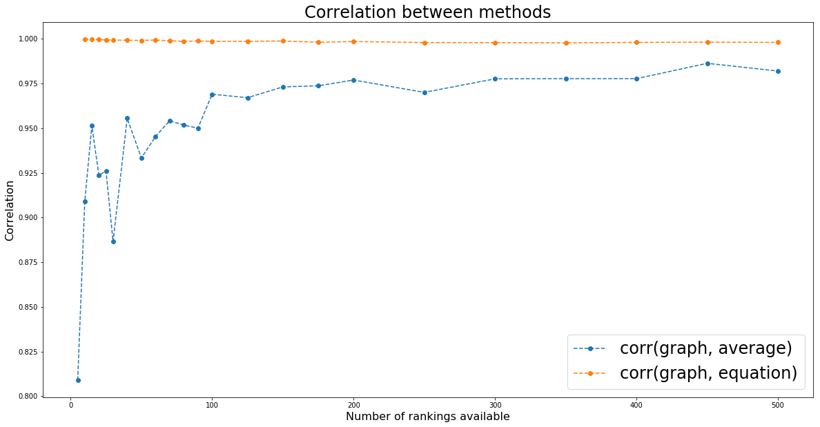
the naive random walking and solving the linear equation give very close solution (correl ~= 0.99+); Since we use a fixed number of steps for the random walking, it should approximate less well for bigger graphs (more rankings to combine): We indeed notice that correlation between the two methods decrease slightly.
-
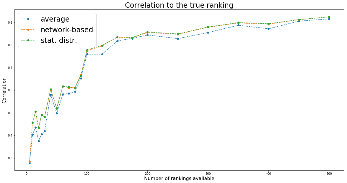
solving the equation yields better results (with respect to the true ranking) than random walking the graph;
-
solving the equation is faster
In the next blog, we will show that with some math we can do potentially even better.
import pandas as pd
import numpy as np
import networkx as nx
from scipy.linalg import block_diag
import matplotlib.pyplot as plt
%matplotlib inline

np.random.seed(seed=42)
def compute_stationary_distribution(P):
    """Returns the stationary distribution of the markov chain.

       Solves x = xP, where x is the stationary distribution.

       x - xP = 0 <-> x(I - P) = 0, such that sum(x) = 1

       :param P: The transition matrix of the markov chain.
    """
    n = P.shape[0]
    # formulates as a x = b
    a = np.eye(n) - P
    a = np.vstack((a.T, np.ones(n)))
    b = np.matrix([0] * n + [1]).T

    return np.linalg.lstsq(a, b)[0]
def build_graph(rankings):
    rank_graph = nx.DiGraph()
    for ranking, ic in rankings:
        for node in ranking.values():
            rank_graph.add_node(node)
    for ranking, ic in rankings:
        for rank_up in range(1, len(ranking)):
            for rank_dn in range(rank_up + 1, len(ranking) + 1):
                u = ranking[rank_up]
                v = ranking[rank_dn]

                if u in rank_graph and v in rank_graph[u]:
                    rank_graph.edges[u, v]['weight'] += ic
                else:
                    rank_graph.add_edge(u, v, weight=ic)

    return rank_graph
def build_markov_chain(rank_graph):
    for node in rank_graph.nodes():
        sum_weights = 0

        for adj_node in rank_graph[node]:
            sum_weights += rank_graph[node][adj_node]['weight']

        for adj_node in rank_graph[node]:
            rank_graph.edges[node, adj_node]['weight'] /= sum_weights

    return rank_graph
def compute_transition_matrix(rank_graph):
    nb_nodes = len(rank_graph.nodes())
    transitions = pd.DataFrame(np.zeros((nb_nodes, nb_nodes)),
                                     index=rank_graph.nodes(),
                                     columns=rank_graph.nodes())
    for node in rank_graph.nodes():
        for adj_node in rank_graph[node]:
            transitions.set_value(node, adj_node, rank_graph[node][adj_node]['weight'])

    return transitions.div(transitions.sum(axis=1), axis=0)
def random_walk(markov_chain, counts, max_random_steps=1000):
    cur_step = 0
    current_node = graph_nodes[np.random.randint(len(graph_nodes))]
    while cur_step < max_random_steps:
        counts[current_node] += 1
        neighbours = [(adj, markov_chain[current_node][adj]['weight'])
                      for adj in markov_chain[current_node]]

        adj_nodes = [adj for adj, w in neighbours]
        adj_weights = [w for adj, w in neighbours]

        if not adj_nodes:
            return counts

        current_node = np.random.choice(adj_nodes, p=adj_weights)

        cur_step += 1

    return counts
nb_assets = 250
nb_observations = 1 * 252

residual_returns = np.random.multivariate_normal(
    np.zeros(nb_assets), cov=np.eye(nb_assets), size=nb_observations)

residual_returns = pd.DataFrame(residual_returns)
ranked_cumulative_residual_returns = (residual_returns
                                      .sum()
                                      .rank(ascending=False))
nb_experts_available = [
    5, 10, 15, 20, 25, 30, 40, 50,
    60, 70, 80, 90, 100, 125, 150,
    175, 200, 250, 300, 350, 400,
    450, 500,
]

results = {}

for nb_experts in nb_experts_available:

    prediction_rankings = []

    for expert in range(nb_experts):
        confidence = np.random.randint(1, 61) / 100
        pct_coverage = np.random.randint(2, 51) / 100
        expert_coverage = np.random.choice(nb_assets, replace=False,
                                           size=int(nb_assets * pct_coverage))

        predictions = []
        for node in expert_coverage:
            prediction = (confidence * residual_returns[node] +
                          np.sqrt(1 - confidence**2) * np.random.normal(
                              0, np.std(residual_returns[node]), nb_observations))
            predictions.append(prediction)

        expert_predictions = pd.DataFrame(np.array(predictions).T,
                                          columns=expert_coverage)
        ranked_cumulated_predictions = (
            expert_predictions
            .sum()
            .rank(ascending=False))

        prediction_rankings.append(
            ({value: key for key, value in dict(ranked_cumulated_predictions).items()},
             confidence))

    rank_graph = build_graph(prediction_rankings)
    markov_chain = build_markov_chain(rank_graph)

    transition_matrix = compute_transition_matrix(rank_graph)
    stationary_distribution = compute_stationary_distribution(
        transition_matrix.values)

    eq_ranking = (pd.DataFrame(stationary_distribution,
                       index=transition_matrix.columns)[0]
                  .rank(ascending=True))

    graph_nodes = list(markov_chain.nodes())

    max_random_steps = 10000
    counts = {node: 0 for node in graph_nodes}

    nb_jumps = 100
    for jump in range(nb_jumps):
        counts = random_walk(markov_chain, counts, max_random_steps)

    # true ranking
    true_ranking = sorted([(key, value)
                           for key, value in dict(ranked_cumulative_residual_returns).items()],
                          key=lambda x: x[1])
    true_ranking = pd.Series([count for node, count in true_ranking],
                         index=[node for node, count in true_ranking])

    # rank graph method
    final_ranking = sorted([(node, count) for node, count in counts.items()],
                           key=lambda x: x[0])

    graph_ranking = (pd.Series([count for node, count in final_ranking],
                              index=[node for node, count in final_ranking])
                     .rank(ascending=True))

    # average ranking
    rankings = pd.DataFrame(np.nan,
                            columns=sorted(graph_nodes),
                            index=range(len(prediction_rankings)))
    for idrank in range(len(prediction_rankings)):
        for rank, asset in prediction_rankings[idrank][0].items():
            rankings[asset].loc[idrank] = rank / len(prediction_rankings[idrank][0])

    sum_weights = sum([prediction_rankings[idrank][1]
                       for idrank in range(len(prediction_rankings))])
    average_rankings = (rankings
                        .multiply([prediction_rankings[idrank][1] / sum_weights
                                   for idrank in range(len(prediction_rankings))],
                                  axis='rows')
                        .sum(axis=0))

    average_ranking = average_rankings.rank(ascending=True)

    results[nb_experts] = {
        'avg': average_ranking.corr(true_ranking, method='spearman'),
        'graph': graph_ranking.corr(true_ranking, method='spearman'),
        'eq': eq_ranking.corr(true_ranking, method='spearman'),
        'corr_graph_eq': eq_ranking.corr(graph_ranking, method='spearman'),
        'corr_graph_avg': graph_ranking.corr(average_ranking, method='spearman')}

    print('number of rankings available:', nb_experts, '\n')
    print(results[nb_experts])
    print('--------------------------------------\n\n')
/home/gmarti/anaconda3/lib/python3.6/site-packages/ipykernel_launcher.py:8: FutureWarning: set_value is deprecated and will be removed in a future release. Please use .at[] or .iat[] accessors instead

/home/gmarti/anaconda3/lib/python3.6/site-packages/ipykernel_launcher.py:16: FutureWarning: `rcond` parameter will change to the default of machine precision times ``max(M, N)`` where M and N are the input matrix dimensions.
To use the future default and silence this warning we advise to pass `rcond=None`, to keep using the old, explicitly pass `rcond=-1`.
  app.launch_new_instance()


number of rankings available: 5

{'avg': 0.27853952574854235, 'graph': 0.28547681249477147, 'eq': nan, 'corr_graph_eq': nan, 'corr_graph_avg': 0.8089651551730394}
--------------------------------------


number of rankings available: 10

{'avg': 0.40457682993752564, 'graph': 0.4564647991823201, 'eq': 0.45614883843479664, 'corr_graph_eq': 0.9997431945445487, 'corr_graph_avg': 0.909035679936199}
--------------------------------------


number of rankings available: 15

{'avg': 0.4360940536338904, 'graph': 0.5043499822580958, 'eq': 0.5066599300427517, 'corr_graph_eq': 0.9995993002718595, 'corr_graph_avg': 0.951359483622102}
--------------------------------------


number of rankings available: 20

{'avg': 0.3760376326021216, 'graph': 0.43245960348275875, 'eq': 0.4344073345173522, 'corr_graph_eq': 0.9995691447757145, 'corr_graph_avg': 0.9235504620944209}
--------------------------------------


number of rankings available: 25

{'avg': 0.40580425286804583, 'graph': 0.4905025607470833, 'eq': 0.4922087073393173, 'corr_graph_eq': 0.9993341328350343, 'corr_graph_avg': 0.9260998808430752}
--------------------------------------


number of rankings available: 30

{'avg': 0.41952325637210186, 'graph': 0.4808010220716799, 'eq': 0.4831000816013056, 'corr_graph_eq': 0.9992412032767914, 'corr_graph_avg': 0.8865637299008844}
--------------------------------------


number of rankings available: 40

{'avg': 0.5807643642298276, 'graph': 0.6020478303247851, 'eq': 0.6041219219507512, 'corr_graph_eq': 0.9991974262349177, 'corr_graph_avg': 0.955521285101716}
--------------------------------------


number of rankings available: 50

{'avg': 0.4981892190275044, 'graph': 0.5219731406647061, 'eq': 0.5188886862189795, 'corr_graph_eq': 0.9991169770243907, 'corr_graph_avg': 0.9333489495986153}
--------------------------------------


number of rankings available: 60

{'avg': 0.581746651946431, 'graph': 0.6176381137293365, 'eq': 0.6172203715259443, 'corr_graph_eq': 0.9992853637432219, 'corr_graph_avg': 0.9452567890450728}
--------------------------------------


number of rankings available: 70

{'avg': 0.5855959295348726, 'graph': 0.6105042738036655, 'eq': 0.6146790188643019, 'corr_graph_eq': 0.9988932925939572, 'corr_graph_avg': 0.9541415318270277}
--------------------------------------


number of rankings available: 80

{'avg': 0.594238371813949, 'graph': 0.6124775668114719, 'eq': 0.6090817453079249, 'corr_graph_eq': 0.9986162320008296, 'corr_graph_avg': 0.9516971462361637}
--------------------------------------


number of rankings available: 90

{'avg': 0.6528814861037776, 'graph': 0.6685824747911345, 'eq': 0.6644193347093552, 'corr_graph_eq': 0.998760811221577, 'corr_graph_avg': 0.9500023616398802}
--------------------------------------


number of rankings available: 100

{'avg': 0.7592097153554457, 'graph': 0.7748645320253476, 'eq': 0.778316325061201, 'corr_graph_eq': 0.9986045195300323, 'corr_graph_avg': 0.9689776319928975}
--------------------------------------


number of rankings available: 125

{'avg': 0.7592404358469735, 'graph': 0.7952108234565716, 'eq': 0.7979367349877597, 'corr_graph_eq': 0.9985849357294801, 'corr_graph_avg': 0.9670326505446638}
--------------------------------------


number of rankings available: 150

{'avg': 0.8177975327605241, 'graph': 0.8338240303172642, 'eq': 0.8357805404886478, 'corr_graph_eq': 0.9987750175805727, 'corr_graph_avg': 0.973077267208882}
--------------------------------------


number of rankings available: 175

{'avg': 0.8296986511784188, 'graph': 0.8322850589517754, 'eq': 0.8335678970863534, 'corr_graph_eq': 0.9980623020217055, 'corr_graph_avg': 0.9736928506789779}
--------------------------------------


number of rankings available: 200

{'avg': 0.8443116209859357, 'graph': 0.855238237870799, 'eq': 0.8576374021984351, 'corr_graph_eq': 0.9984816367927717, 'corr_graph_avg': 0.9769219544432244}
--------------------------------------


number of rankings available: 250

{'avg': 0.8281987231795707, 'graph': 0.8472580281915887, 'eq': 0.8489627034032543, 'corr_graph_eq': 0.9978931466511936, 'corr_graph_avg': 0.9700315327204603}
--------------------------------------


number of rankings available: 300

{'avg': 0.8552066433062929, 'graph': 0.8782567623628004, 'eq': 0.8796125378006048, 'corr_graph_eq': 0.9978668417756439, 'corr_graph_avg': 0.9775797582310694}
--------------------------------------


number of rankings available: 350

{'avg': 0.8873794460711371, 'graph': 0.8973040454295462, 'eq': 0.8992406278500454, 'corr_graph_eq': 0.9977282187792099, 'corr_graph_avg': 0.9777188029449393}
--------------------------------------


number of rankings available: 400

{'avg': 0.8717043152690442, 'graph': 0.8921848632542332, 'eq': 0.8941863389814236, 'corr_graph_eq': 0.9979787793938781, 'corr_graph_avg': 0.9776978360653875}
--------------------------------------


number of rankings available: 450

{'avg': 0.9056074497191954, 'graph': 0.9119969678836083, 'eq': 0.9122791724667596, 'corr_graph_eq': 0.9981012783409526, 'corr_graph_avg': 0.9862853888688462}
--------------------------------------


number of rankings available: 500

{'avg': 0.9154426150818412, 'graph': 0.9246062443715376, 'eq': 0.9244160706571304, 'corr_graph_eq': 0.9979830050181402, 'corr_graph_avg': 0.9819553350342176}
--------------------------------------
plt.figure(figsize=(20, 10))
plt.plot(nb_experts_available,
         [results[nb_experts]['avg'] for nb_experts in nb_experts_available],
         '--o', label='average')
plt.plot(nb_experts_available,
         [results[nb_experts]['graph'] for nb_experts in nb_experts_available],
         '--o', label='network-based')
plt.plot(nb_experts_available,
         [results[nb_experts]['eq'] for nb_experts in nb_experts_available],
         '--o', label='stat. distr.')
plt.title('Correlation to the true ranking', fontsize=24)
plt.legend(fontsize=24)
plt.xlabel('Number of rankings available', fontsize=16)
plt.ylabel('Correlation', fontsize=16)
plt.show()
plt.figure(figsize=(20, 10))
plt.plot(nb_experts_available,
         [results[nb_experts]['corr_graph_avg'] for nb_experts in nb_experts_available],
         '--o', label='corr(graph, average)')
plt.plot(nb_experts_available,
         [results[nb_experts]['corr_graph_eq'] for nb_experts in nb_experts_available],
         '--o', label='corr(graph, equation)')
plt.title('Correlation between methods', fontsize=24)
plt.legend(fontsize=24)
plt.xlabel('Number of rankings available', fontsize=16)
plt.ylabel('Correlation', fontsize=16)
plt.show()