CorrGAN: A GAN for sampling correlation matrices (Part I)
CorrGAN: A GAN for sampling correlation matrices (Part I)
In a previous blog, we exposed how to sample uniformly over the space of correlation matrices. In practice, we may want to sample from a subset of the space of correlation matrices (also called elliptope), which is not clearly defined, but implicitely defined by empirical observations. Generative adversarial networks (GANs) may be a good option to sample from this ‘not well specified subspace’. For example, GANs have been found successful for sampling from the ‘human faces’ subspace of ‘natural images’ subspace of all possible colored images (matrices/tensors) (cf. StyleGAN). The ‘human faces’ and ‘natural images’ subspaces are not formally defined, we only have an understanding of them through many examples.
Before trying to sample from any ‘complex’ subset of the N-dimensional elliptope, let’s focus on the full 3-dimensional elliptope (which corresponds to the set of 3x3 correlation matrices). At least,
- we know how to sample (uniformly) perfectly from the elliptope so that we can compare with the samples generated by the GAN,
- we can visualize the results in 3D.
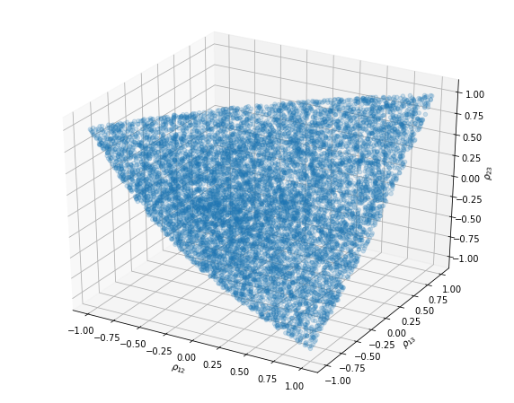
Below some code that allows to sample nearly correctly from the 3D elliptope. Notice that a few points are living outside the hull. They correspond to 3x3 matrices which are not positive semidefinite (hence not proper correlation matrices). Notice that, here, we generate only 3 coefficients since out of the 3x3=9 coefficient, only n(n-1)/2 = 3 matters (3 being forced to 1 (diagonal), 3 are defined by the symmetry). We could ask the GAN to learn the diagonal property (=1) and the symmetry property (C = C^T), but that would make the problem uselessly harder.
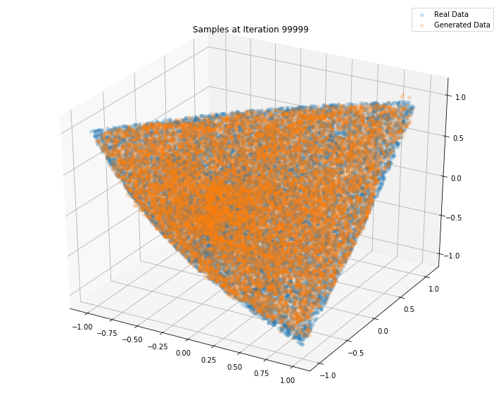
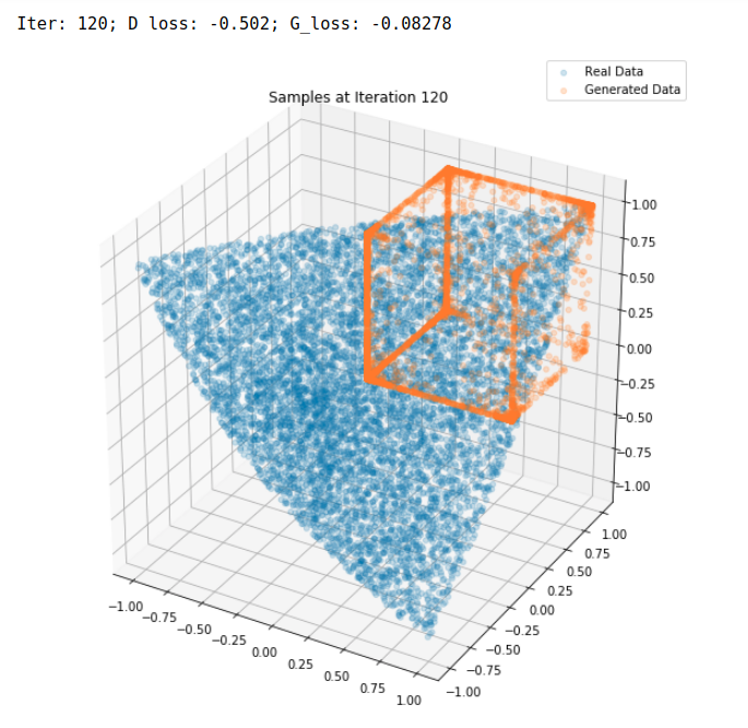
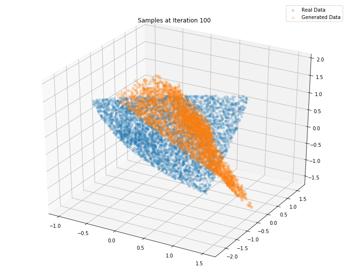
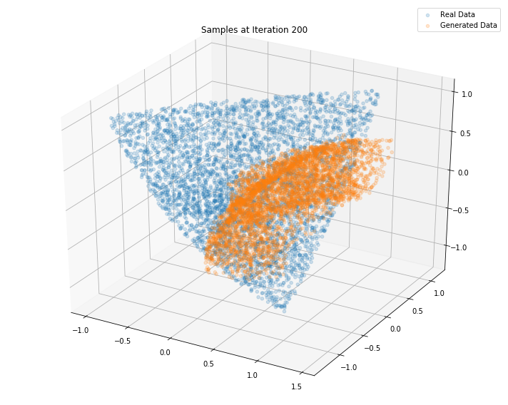
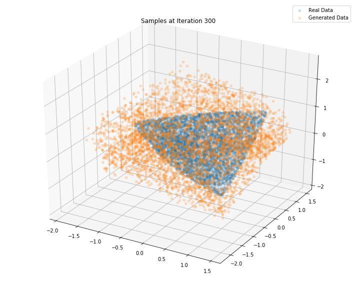
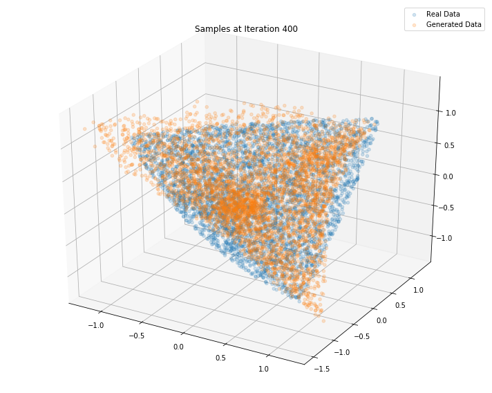
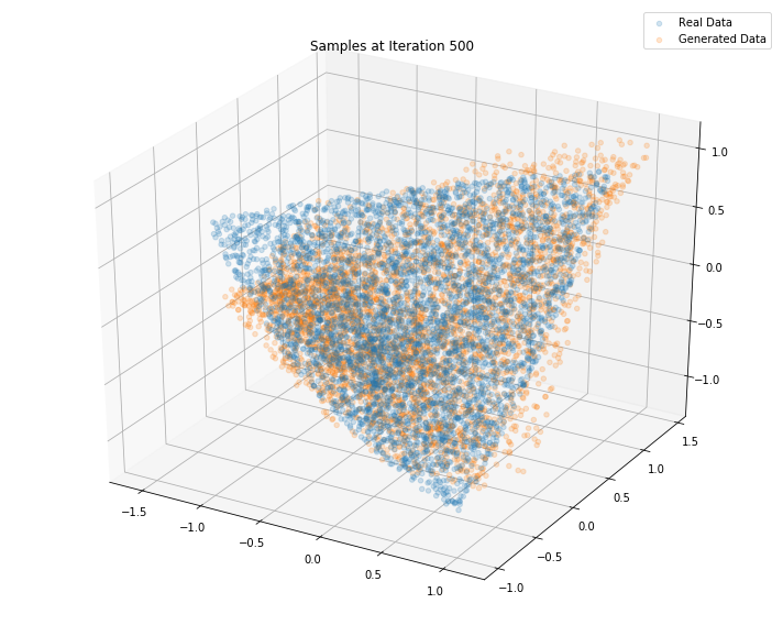
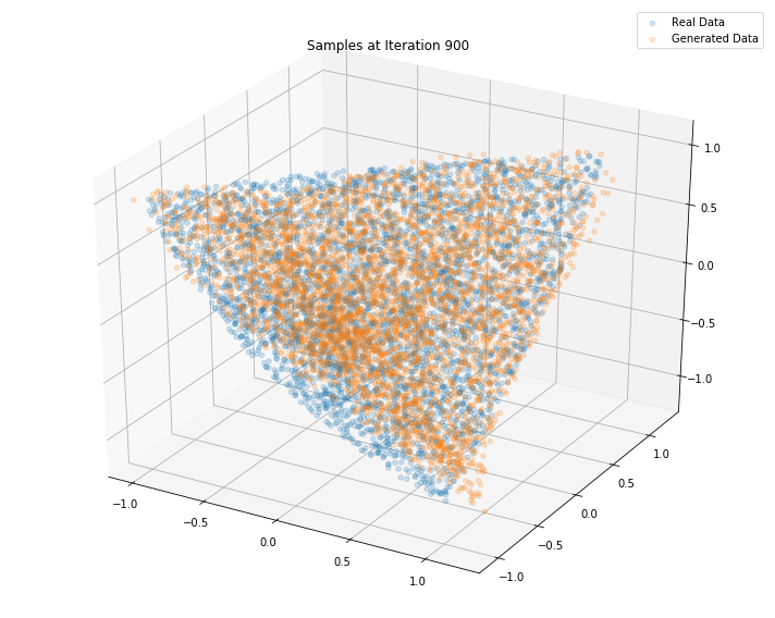
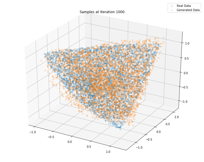
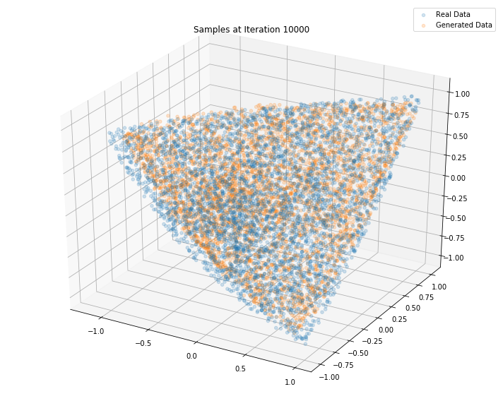
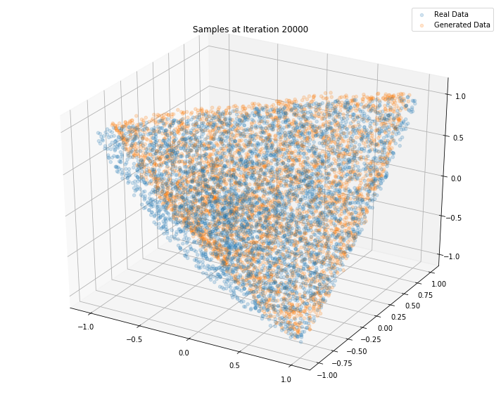
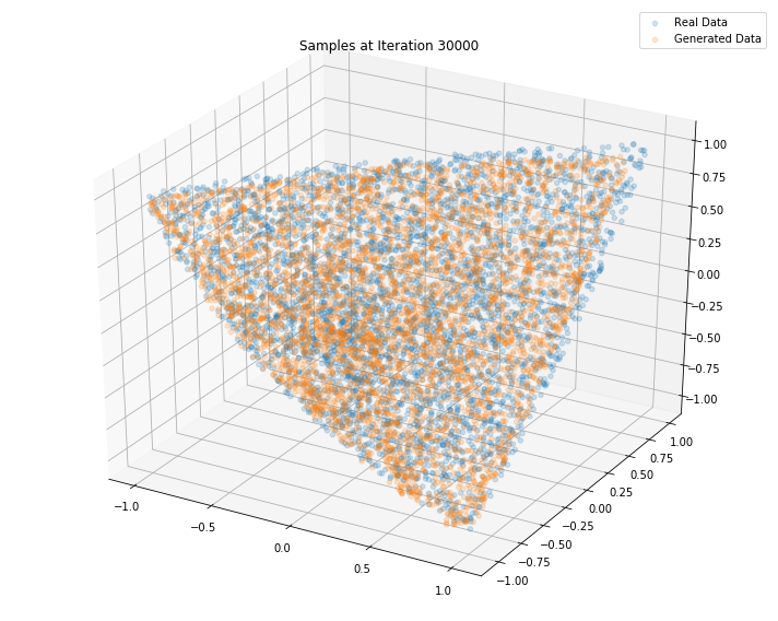
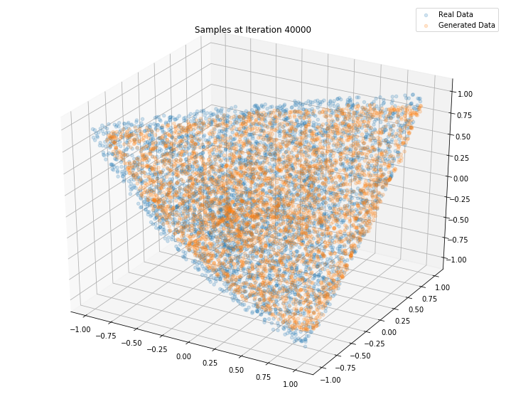
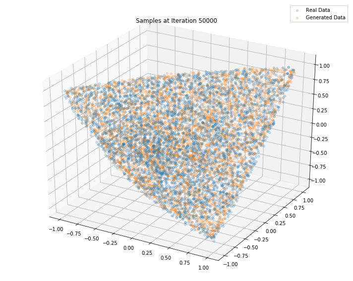
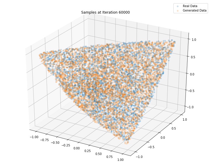
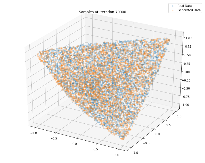
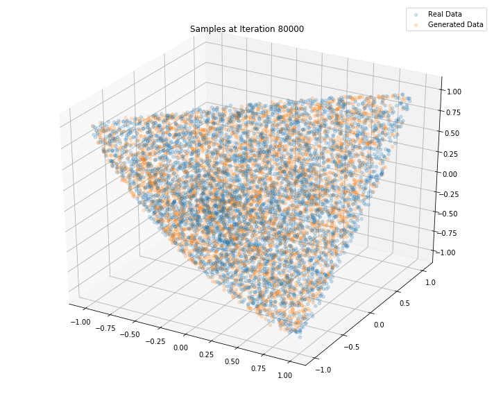
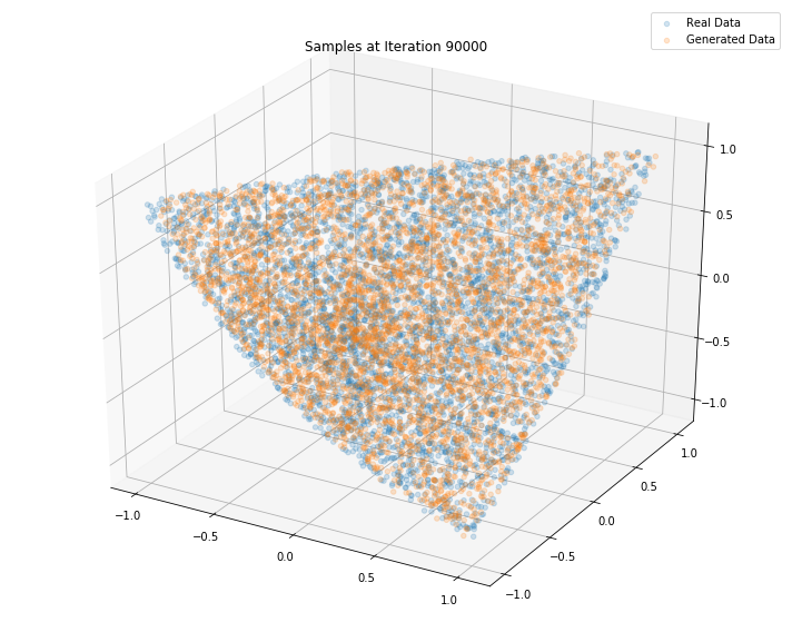
TL;DR (Left) Generated samples from vanilla GAN (in orange); (Right) Generated samples from Wasserstein GAN (in orange). Something went wrong… What?
import numpy as np
from numpy.random import beta
from numpy.random import randn
from scipy.linalg import sqrtm
from numpy.random import seed

seed(42)


def sample_unif_correlmat(dimension):
    d = dimension + 1

    prev_corr = np.matrix(np.ones(1))
    for k in range(2, d):
        # sample y = r^2 from a beta distribution with alpha_1 = (k-1)/2 and alpha_2 = (d-k)/2
        y = beta((k - 1) / 2, (d - k) / 2)
        r = np.sqrt(y)

        # sample a unit vector theta uniformly from the unit ball surface B^(k-1)
        v = randn(k-1)
        theta = v / np.linalg.norm(v)

        # set w = r theta
        w = np.dot(r, theta)

        # set q = prev_corr**(1/2) w
        q = np.dot(sqrtm(prev_corr), w)

        next_corr = np.zeros((k, k))
        next_corr[:(k-1), :(k-1)] = prev_corr
        next_corr[k-1, k-1] = 1
        next_corr[k-1, :(k-1)] = q
        next_corr[:(k-1), k-1] = q

        prev_corr = next_corr

    return next_corr
sample_unif_correlmat(3)
array([[ 1.        ,  0.36739638,  0.1083456 ],
       [ 0.36739638,  1.        , -0.05167306],
       [ 0.1083456 , -0.05167306,  1.        ]])
def sample_data(n=10000):
    data = []
    for i in range(n):
        m = sample_unif_correlmat(3)
        data.append([m[0, 1], m[0, 2], m[1, 2]])

    return np.array(data)
from mpl_toolkits.mplot3d import Axes3D
import matplotlib.pyplot as plt


fig = plt.figure(figsize=(10, 8))
ax = fig.add_subplot(111, projection='3d')

xs = []
ys = []
zs = []
d = sample_data()
for datum in d:
    xs.append(datum[0])
    ys.append(datum[1])
    zs.append(datum[2])

ax.scatter(xs, ys, zs, alpha=0.2)

ax.set_xlabel('$\\rho_{12}$')
ax.set_ylabel('$\\rho_{13}$')
ax.set_zlabel('$\\rho_{23}$')

plt.show()
import tensorflow as tf
import keras
Using TensorFlow backend.
def generator(Z, hsize=[64, 64, 16], reuse=False):
    with tf.variable_scope("GAN/Generator", reuse=reuse):
        h1 = tf.layers.dense(Z, hsize[0], activation=tf.nn.leaky_relu)
        h2 = tf.layers.dense(h1, hsize[1], activation=tf.nn.leaky_relu)
        h3 = tf.layers.dense(h2, hsize[2], activation=tf.nn.leaky_relu)
        out = tf.layers.dense(h3, 3)

    return out
def discriminator(X, hsize=[64, 64, 16], reuse=False):
    with tf.variable_scope("GAN/Discriminator", reuse=reuse):
        h1 = tf.layers.dense(X, hsize[0], activation=tf.nn.leaky_relu)
        h2 = tf.layers.dense(h1, hsize[1], activation=tf.nn.leaky_relu)
        h3 = tf.layers.dense(h2, hsize[2], activation=tf.nn.leaky_relu)
        h4 = tf.layers.dense(h3, 3)
        out = tf.layers.dense(h4, 1)

    return out, h4
X = tf.placeholder(tf.float32, [None, 3])
Z = tf.placeholder(tf.float32, [None, 3])
G_sample = generator(Z)
r_logits, r_rep = discriminator(X)
f_logits, g_rep = discriminator(G_sample, reuse=True)
disc_loss = tf.reduce_mean(
    tf.nn.sigmoid_cross_entropy_with_logits(
        logits=r_logits, labels=tf.ones_like(r_logits))
    + tf.nn.sigmoid_cross_entropy_with_logits(
        logits=f_logits, labels=tf.zeros_like(f_logits)))

gen_loss = tf.reduce_mean(
    tf.nn.sigmoid_cross_entropy_with_logits(
        logits=f_logits, labels=tf.ones_like(f_logits)))
gen_vars = tf.get_collection(tf.GraphKeys.GLOBAL_VARIABLES, scope="GAN/Generator")
disc_vars = tf.get_collection(tf.GraphKeys.GLOBAL_VARIABLES, scope="GAN/Discriminator")

gen_step = tf.train.RMSPropOptimizer(
    learning_rate=0.0001).minimize(gen_loss, var_list=gen_vars)
disc_step = tf.train.RMSPropOptimizer(
    learning_rate=0.0001).minimize(disc_loss, var_list=disc_vars)
sess = tf.Session()
tf.global_variables_initializer().run(session=sess)

batch_size = 2**8
nd_steps = 5
ng_steps = 5
def sample_Z(m, n):
    return np.random.uniform(-1., 1., size=[m, n])

n_dots = 2**12
x_plot = sample_data(n=n_dots)
Z_plot = sample_Z(n_dots, 3)
for i in range(100000):
X_batch = sample_data(n=batch_size)
Z_batch = sample_Z(batch_size, 3)
for _ in range(nd_steps):
_, dloss = sess.run([disc_step, disc_loss], feed_dict={X: X_batch, Z: Z_batch})
rrep_dstep, grep_dstep = sess.run([r_rep, g_rep], feed_dict={X: X_batch, Z: Z_batch})
for _ in range(ng_steps):
_, gloss = sess.run([gen_step, gen_loss], feed_dict={Z: Z_batch})
rrep_gstep, grep_gstep = sess.run([r_rep, g_rep], feed_dict={X: X_batch, Z: Z_batch})
if (i <= 1000 and i % 100 == 0) or (i % 10000 == 0):
print("Iterations: %d\t Discriminator loss: %.4f\t Generator loss: %.4f"%(i, dloss, gloss))
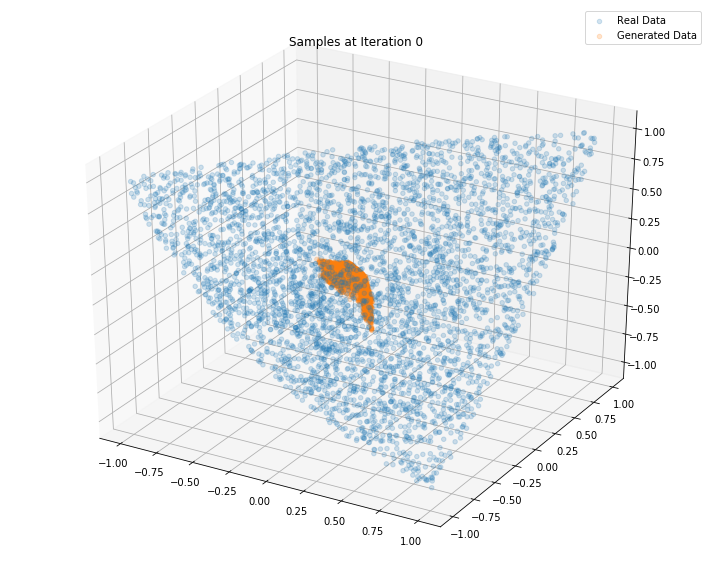
fig = plt.figure(figsize=(10, 8))
g_plot = sess.run(G_sample, feed_dict={Z: Z_plot})
ax = fig.add_subplot(111, projection='3d')
ax.scatter(x_plot[:, 0], x_plot[:, 1], x_plot[:, 2], alpha=0.2)
ax.scatter(g_plot[:, 0], g_plot[:, 1], g_plot[:, 2], alpha=0.2)
plt.legend(["Real Data", "Generated Data"])
plt.title('Samples at Iteration %d' % i)
plt.tight_layout()
plt.show()
plt.close()
Iterations: 0 Discriminator loss: 1.3821 Generator loss: 0.6854
Iterations: 100 Discriminator loss: 1.3222 Generator loss: 0.7560
Iterations: 200 Discriminator loss: 1.4604 Generator loss: 0.6441
Iterations: 300 Discriminator loss: 1.3710 Generator loss: 0.8039
Iterations: 400 Discriminator loss: 1.3793 Generator loss: 0.7000
Iterations: 500 Discriminator loss: 1.3865 Generator loss: 0.6892
Iterations: 600 Discriminator loss: 1.3851 Generator loss: 0.7015
Iterations: 700 Discriminator loss: 1.3903 Generator loss: 0.6932
Iterations: 800 Discriminator loss: 1.3854 Generator loss: 0.6958
Iterations: 900 Discriminator loss: 1.3836 Generator loss: 0.6837
Iterations: 1000 Discriminator loss: 1.3881 Generator loss: 0.6930
Iterations: 10000 Discriminator loss: 1.3806 Generator loss: 0.7006
Iterations: 20000 Discriminator loss: 1.3824 Generator loss: 0.6903
Iterations: 30000 Discriminator loss: 1.3694 Generator loss: 0.6960
Iterations: 40000 Discriminator loss: 1.3579 Generator loss: 0.6888
Iterations: 50000 Discriminator loss: 1.3454 Generator loss: 0.6856
Iterations: 60000 Discriminator loss: 1.3551 Generator loss: 0.7187
Iterations: 70000 Discriminator loss: 1.3141 Generator loss: 0.7412
Iterations: 80000 Discriminator loss: 1.2773 Generator loss: 0.7295
Iterations: 90000 Discriminator loss: 1.3026 Generator loss: 0.7882
n_dots = 2**14
x_plot = sample_data(n=n_dots)
Z_plot = sample_Z(n_dots, 3)

fig = plt.figure(figsize=(10, 8))
g_plot = sess.run(G_sample, feed_dict={Z: Z_plot})
ax = fig.add_subplot(111, projection='3d')
ax.scatter(x_plot[:, 0], x_plot[:, 1], x_plot[:, 2], alpha=0.2)
ax.scatter(g_plot[:, 0], g_plot[:, 1], g_plot[:, 2], alpha=0.2)

plt.legend(["Real Data", "Generated Data"])
plt.title('Samples at Iteration %d' % i)
plt.tight_layout()
plt.show()
plt.close()
Conclusion: This simple GAN is quite useless in practice as it learns how to sample from a distribution for which we already have a good sampling algorithm, namely the onion method. However, it is an interesting exercise to see what it takes to replicate it with a GAN approach. Since successful, we envision to sample from much more complex distributions such as the distribution of “empirical financial correlation matrices” for which no sampling algorithms are known.