CorrGAN: A GAN for sampling correlation matrices (Part II)
CorrGAN: A GAN for sampling correlation matrices (Part II)
In this blog, we do a tiny step toward the ultimate goal of sampling realistic financial correlation matrices thanks to a GAN.
For this experiment, we still restrain ourselves to 3x3 correlation matrices (as we can easily visualize them in a 3D space), but instead of learning to sample from the full 3D elliptope like in (Part I), we try to learn to sample from the 3x3 subspace of realistic financial correlation matrices.
By subspace of “realistic financial correlation matrices”, we mean the space loosely defined by millions of 3x3 empirical correlation matrices estimated on returns of the S&P500 constituents.
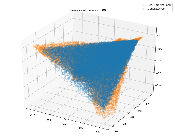
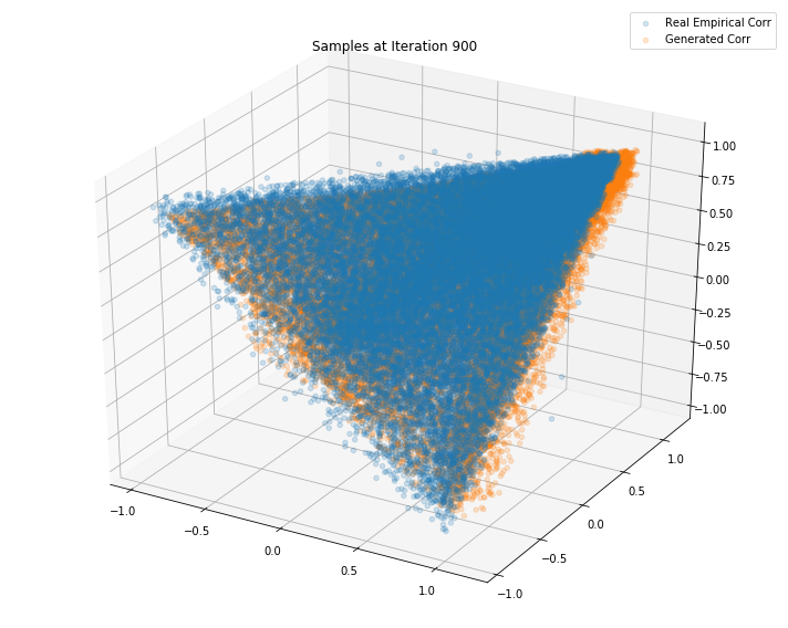
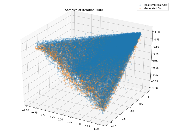
TL;DR It seems that the GAN do a decent job at sampling correlation matrices that could have been estimated from real returns of S&P500 constituents.
Next steps:
-
Since in N-dimensions we cannot visualize easily anymore, we can try to compare the two orbifolds (original one vs. learned by GAN one) using Topological Data Analysis metrics (as in https://arxiv.org/pdf/1802.02664.pdf): Hopefully, the numbers closely match meaning the GAN might cover rather the whole subspace;
-
We can monitor a few summary statistics about the GAN-generated correlation matrices, and check whether they verify the “stylized facts” (1. Large first eigenvalue, 2. Perron-Frobenius property, 3. Eigenvalues follow the Marchenko–Pastur distribution 4. Distribution of pairwise correlations is signicantly shifted to the positive, 5. Scale-free property of the corresponding MST, 6. Hierarchical structure of clusters) known in the finance literature: This will tell if they are realistic, but not that the GAN cover the whole subspace;
-
Modify the neural networks so that they verify the exchangeability property, i.e. f(x1, x2, …, xn) = f(p(x1), p(x2), …, p(xn)), where p is a permutation of the n variables. Indeed, the order of the rows (and columns) of the correlation matrix is totally arbitrary (corr(A, B, C) should be equivalent to corr(B, C, A)). So, n! equivalent correlation matrices. For the 3x3, it’s not blocking as we can naively sample many equivalent matrices, but exchangeability is not an option for higher dimensions (https://arxiv.org/pdf/1703.06114.pdf).
import pandas as pd
import numpy as np
from numpy.random import beta
from numpy.random import randn
from scipy.linalg import sqrtm
from numpy.random import seed
from random import randint

seed(42)


def sample_unif_correlmat(dimension):
    d = dimension + 1

    prev_corr = np.matrix(np.ones(1))
    for k in range(2, d):
        # sample y = r^2 from a beta distribution with alpha_1 = (k-1)/2 and alpha_2 = (d-k)/2
        y = beta((k - 1) / 2, (d - k) / 2)
        r = np.sqrt(y)

        # sample a unit vector theta uniformly from the unit ball surface B^(k-1)
        v = randn(k-1)
        theta = v / np.linalg.norm(v)

        # set w = r theta
        w = np.dot(r, theta)

        # set q = prev_corr**(1/2) w
        q = np.dot(sqrtm(prev_corr), w)

        next_corr = np.zeros((k, k))
        next_corr[:(k-1), :(k-1)] = prev_corr
        next_corr[k-1, k-1] = 1
        next_corr[k-1, :(k-1)] = q
        next_corr[:(k-1), k-1] = q

        prev_corr = next_corr

    return next_corr
sample_unif_correlmat(3)
array([[ 1.        ,  0.36739638,  0.1083456 ],
       [ 0.36739638,  1.        , -0.05167306],
       [ 0.1083456 , -0.05167306,  1.        ]])
We load a total of more than 25 million 3x3 empirical correlation matrices that were estimated on returns of the S&P500 constituents. We want the GAN to learn their distribution.
corrs = pd.read_hdf('corr_emp_3d.h5')
corrs.shape
(25898310, 3)
def sample_data(n=10000):
    data = []
    for i in range(n):
        m = sample_unif_correlmat(3)
        data.append([m[0, 1], m[0, 2], m[1, 2]])

    return np.array(data)


def sample_corr(n=10000):
    idx = [randint(0, len(corrs) - 1) for j in range(n)]

    return corrs.loc[idx].values
from mpl_toolkits.mplot3d import Axes3D
import matplotlib.pyplot as plt


fig = plt.figure(figsize=(10, 8))
ax = fig.add_subplot(111, projection='3d')

xs = []
ys = []
zs = []
d = sample_data()
for datum in d:
    xs.append(datum[0])
    ys.append(datum[1])
    zs.append(datum[2])

xc = []
yc = []
zc = []
c = sample_corr()
for corr in c:
    xc.append(corr[0])
    yc.append(corr[1])
    zc.append(corr[2])

ax.scatter(xs, ys, zs, alpha=0.1)
ax.scatter(xc, yc, zc, alpha=0.2)

ax.set_xlabel('$\\rho_{12}$')
ax.set_ylabel('$\\rho_{13}$')
ax.set_zlabel('$\\rho_{23}$')

ax.legend(['elliptope', 'emprical corr mats'])

plt.show()
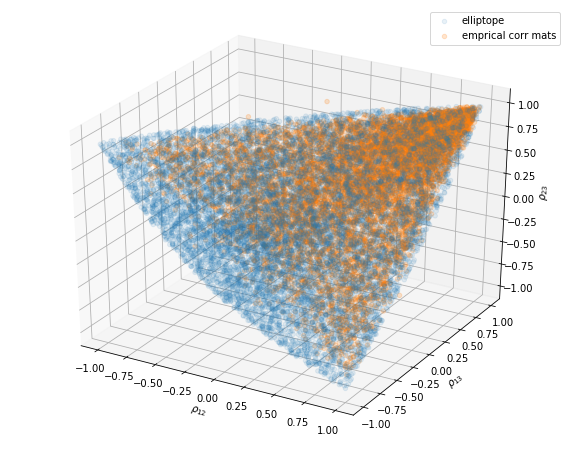
Note that some of the empirical correlation matrices are actually not proper correlation matrices as they live out of the elliptope (they are not positive semidefinite).
import tensorflow as tf
import keras
Using TensorFlow backend.
def generator(Z, hsize=[64, 64, 16], reuse=False):
    with tf.variable_scope("GAN/Generator", reuse=reuse):
        h1 = tf.layers.dense(Z, hsize[0], activation=tf.nn.leaky_relu)
        h2 = tf.layers.dense(h1, hsize[1], activation=tf.nn.leaky_relu)
        h3 = tf.layers.dense(h2, hsize[2], activation=tf.nn.leaky_relu)
        out = tf.layers.dense(h3, 3)

    return out
def discriminator(X, hsize=[64, 64, 16], reuse=False):
    with tf.variable_scope("GAN/Discriminator", reuse=reuse):
        h1 = tf.layers.dense(X, hsize[0], activation=tf.nn.leaky_relu)
        h2 = tf.layers.dense(h1, hsize[1], activation=tf.nn.leaky_relu)
        h3 = tf.layers.dense(h2, hsize[2], activation=tf.nn.leaky_relu)
        h4 = tf.layers.dense(h3, 3)
        out = tf.layers.dense(h4, 1)

    return out, h4
X = tf.placeholder(tf.float32, [None, 3])
Z = tf.placeholder(tf.float32, [None, 3])
G_sample = generator(Z)
r_logits, r_rep = discriminator(X)
f_logits, g_rep = discriminator(G_sample, reuse=True)
disc_loss = tf.reduce_mean(
    tf.nn.sigmoid_cross_entropy_with_logits(
        logits=r_logits, labels=tf.ones_like(r_logits))
    + tf.nn.sigmoid_cross_entropy_with_logits(
        logits=f_logits, labels=tf.zeros_like(f_logits)))

gen_loss = tf.reduce_mean(
    tf.nn.sigmoid_cross_entropy_with_logits(
        logits=f_logits, labels=tf.ones_like(f_logits)))
gen_vars = tf.get_collection(tf.GraphKeys.GLOBAL_VARIABLES, scope="GAN/Generator")
disc_vars = tf.get_collection(tf.GraphKeys.GLOBAL_VARIABLES, scope="GAN/Discriminator")

gen_step = tf.train.RMSPropOptimizer(
    learning_rate=0.0001).minimize(gen_loss, var_list=gen_vars)
disc_step = tf.train.RMSPropOptimizer(
    learning_rate=0.0001).minimize(disc_loss, var_list=disc_vars)
sess = tf.Session()
tf.global_variables_initializer().run(session=sess)

batch_size = 2**9
nd_steps = 5
ng_steps = 5
def sample_Z(m, n):
    return np.random.uniform(-1., 1., size=[m, n])

n_dots = 2**15
x_plot = sample_corr(n=n_dots)
Z_plot = sample_Z(n_dots, 3)
for i in range(200000 + 1):
X_batch = sample_corr(n=batch_size)
Z_batch = sample_Z(batch_size, 3)
for _ in range(nd_steps):
_, dloss = sess.run([disc_step, disc_loss], feed_dict={X: X_batch, Z: Z_batch})
rrep_dstep, grep_dstep = sess.run([r_rep, g_rep], feed_dict={X: X_batch, Z: Z_batch})
for _ in range(ng_steps):
_, gloss = sess.run([gen_step, gen_loss], feed_dict={Z: Z_batch})
rrep_gstep, grep_gstep = sess.run([r_rep, g_rep], feed_dict={X: X_batch, Z: Z_batch})
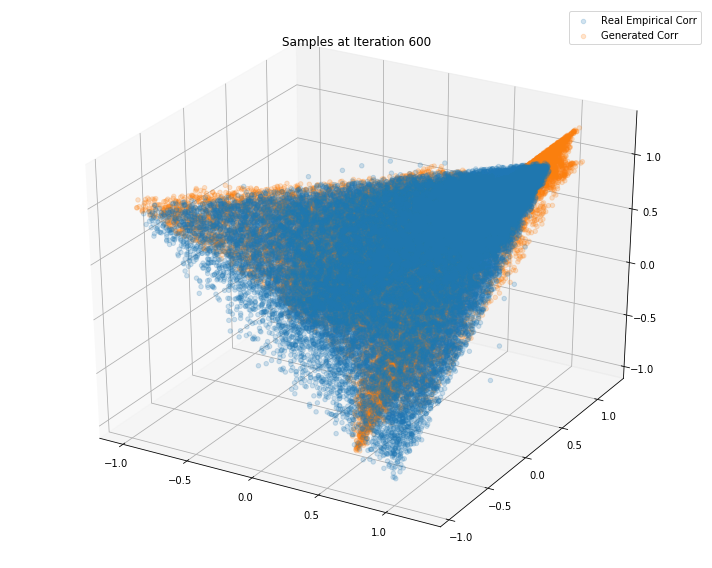
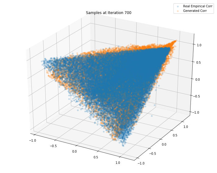
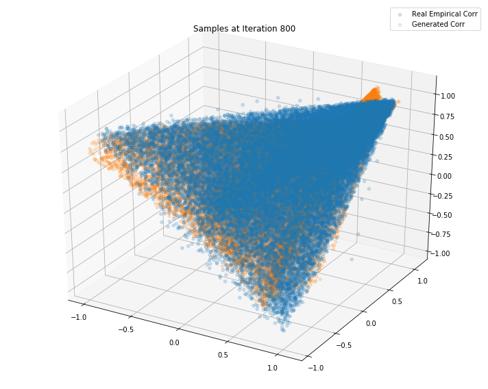
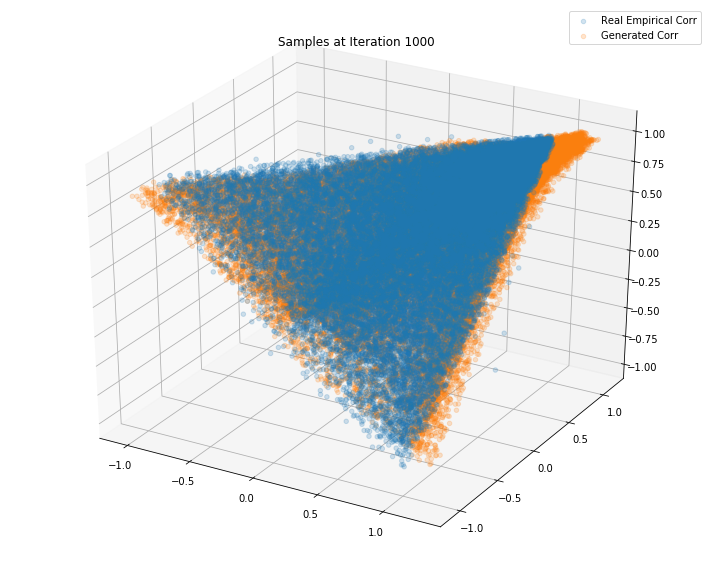
if (i <= 1000 and i % 100 == 0) or (i % 10000 == 0):
print("Iterations: %d\t Discriminator loss: %.4f\t Generator loss: %.4f"%(i, dloss, gloss))
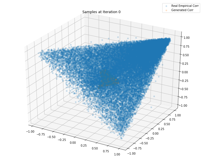
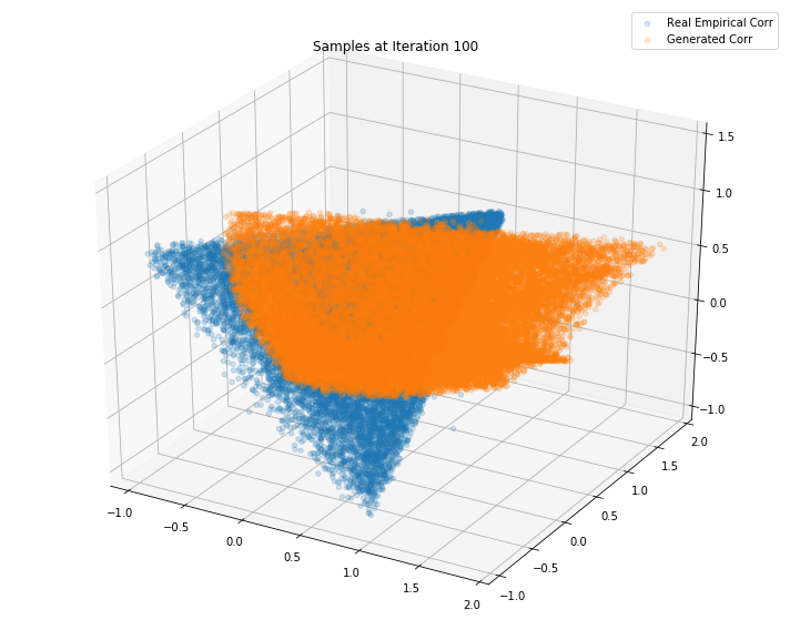
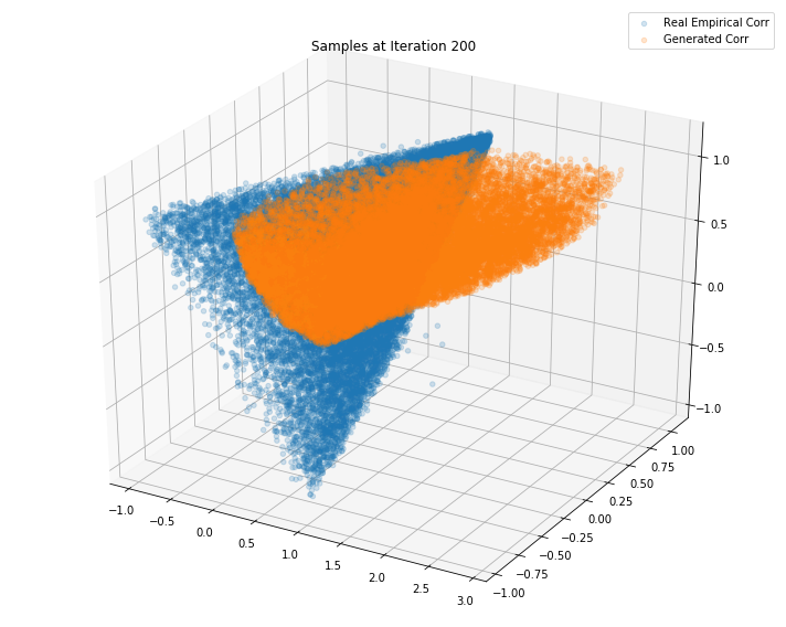
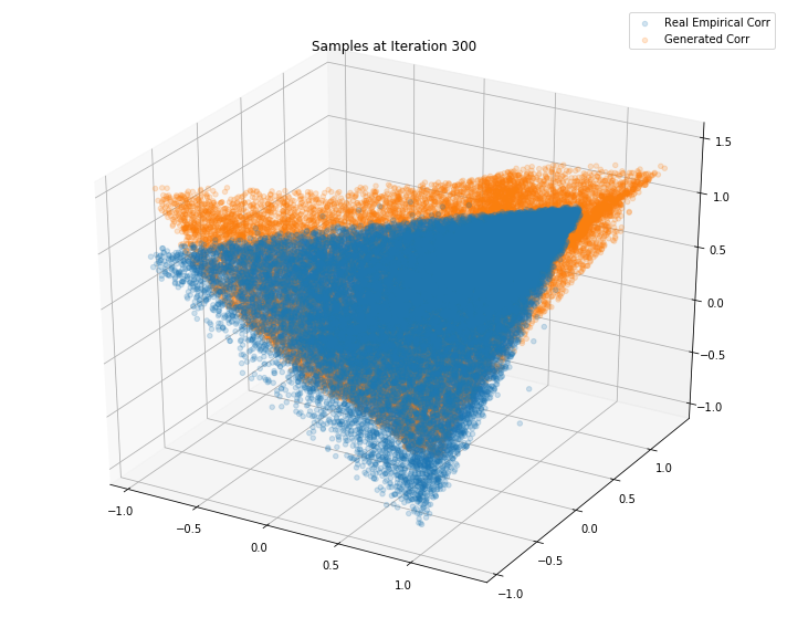
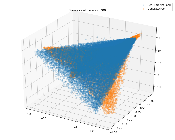
fig = plt.figure(figsize=(10, 8))
g_plot = sess.run(G_sample, feed_dict={Z: Z_plot})
ax = fig.add_subplot(111, projection='3d')
ax.scatter(x_plot[:, 0], x_plot[:, 1], x_plot[:, 2], alpha=0.2)
ax.scatter(g_plot[:, 0], g_plot[:, 1], g_plot[:, 2], alpha=0.2)
plt.legend(["Real Empirical Corr", "Generated Corr"])
plt.title('Samples at Iteration %d' % i)
plt.tight_layout()
plt.show()
plt.close()
Iterations: 0 Discriminator loss: 1.3851 Generator loss: 0.6945
Iterations: 100 Discriminator loss: 1.2771 Generator loss: 0.7747
Iterations: 200 Discriminator loss: 1.4413 Generator loss: 0.6601
Iterations: 300 Discriminator loss: 1.3758 Generator loss: 0.7050
Iterations: 400 Discriminator loss: 1.3885 Generator loss: 0.6952
Iterations: 500 Discriminator loss: 1.3843 Generator loss: 0.7001
Iterations: 600 Discriminator loss: 1.3835 Generator loss: 0.6997
Iterations: 700 Discriminator loss: 1.3832 Generator loss: 0.7047
Iterations: 800 Discriminator loss: 1.3851 Generator loss: 0.6845
Iterations: 900 Discriminator loss: 1.3841 Generator loss: 0.7035
Iterations: 1000 Discriminator loss: 1.3850 Generator loss: 0.6881
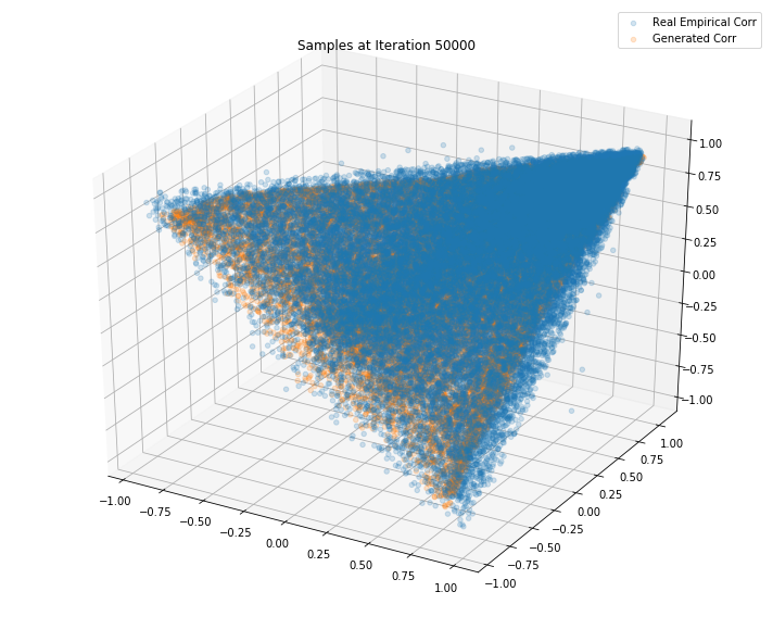
Iterations: 50000 Discriminator loss: 1.3858 Generator loss: 0.6898
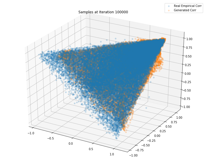
Iterations: 100000 Discriminator loss: 1.3795 Generator loss: 0.6682
Iterations: 150000 Discriminator loss: 1.3700 Generator loss: 0.6214
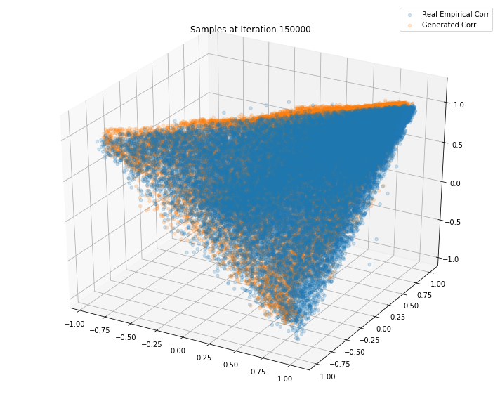
Iterations: 200000 Discriminator loss: 1.3853 Generator loss: 0.7050
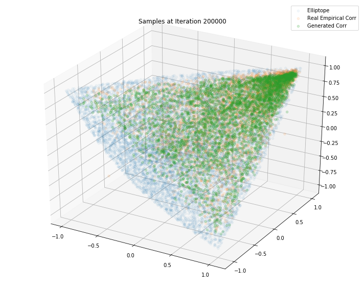
n_dots = 2**12
x_plot = sample_corr(n=n_dots)
Z_plot = sample_Z(n_dots, 3)

fig = plt.figure(figsize=(10, 8))
g_plot = sess.run(G_sample, feed_dict={Z: Z_plot})
ax = fig.add_subplot(111, projection='3d')

ax.scatter(xs, ys, zs, alpha=0.05)
ax.scatter(x_plot[:, 0], x_plot[:, 1], x_plot[:, 2], alpha=0.1)
ax.scatter(g_plot[:, 0], g_plot[:, 1], g_plot[:, 2], alpha=0.2)

plt.legend(["Elliptope", "Real Empirical Corr", "Generated Corr"])
plt.title('Samples at Iteration %d' % i)
plt.tight_layout()
plt.show()
plt.close()