TF 2.0 GAN MLP for 100x100 financial correlation matrices
TF 2.0 GAN MLP for 100x100 financial correlation matrices
Give it some time for the animation below (heavy gif) to start (~30s):
 A few correlation matrices generated by the GAN, evolving during the iterative training process. From random noise to some structured matrix.
TL;DR This is an attempt toward a GAN for generating realistic financial correlation matrices. We are not there yet: Stylized facts (as described in this previous blog) are not verified.
For this blog, we will use TensorFlow 2.0, and play around with this DCGAN tutorial.
import tensorflow as tf

tf.__version__
'2.0.0-rc1'
%matplotlib inline

import os
import time
import glob
import imageio
import matplotlib.pyplot as plt
import pandas as pd
import numpy as np
import fastcluster
import networkx as nx
from scipy.cluster import hierarchy
import PIL
from tensorflow.keras import layers

from IPython import display
Because of the huge number of equivalent matrices (cf. this previous blog on permutation invariance in the context of correlation matrices), we re-order the correlation matrices using the following:
def canonical_repr(corr):
    permutation = corr.sum(axis=1).argsort()
    prows = corr[permutation, :]
    perm = prows[:, permutation]

    return perm
We will generate using the GAN only the upper triangular matrix, that is n * (n - 1) /2 coefficients. We are enforcing diag = 1 and the symmetry post-generation of the upper triangular.
n = 100
a, b = np.triu_indices(n, k=1)

corrs = []
for r, d, files in os.walk('sorted_corrs/'):
    for file in files:
        if 'corr_emp_{}d_batch_'.format(n) in file:
            flat_corr = pd.read_hdf('sorted_corrs/{}'.format(file))
            corr = np.ones((n, n))
            corr[a, b] = flat_corr
            corr[b, a] = flat_corr
            canon_repr = canonical_repr(corr)
            corrs.append(canon_repr[a, b])
corrs = (np
         .array(corrs)
         .reshape(len(corrs), int(n * (n - 1) / 2))
         .astype('float32'))
corrs.shape
(9196, 4950)
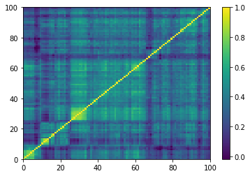
idx = 0
plt.plot(corrs[idx, :])
plt.show()

c = np.ones((n, n))
c[a, b] = corrs[idx, :]
c[b, a] = corrs[idx, :]

plt.pcolormesh(c)
plt.colorbar()
plt.show()
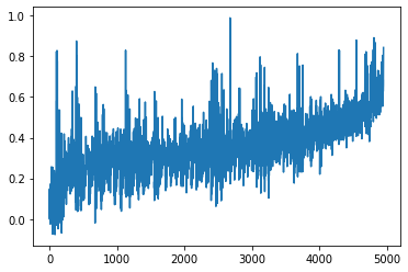
The n * (n - 1) / 2 = 4950 coefficients. These coefficients are real empirical pairwise correlations estimated from 100 time series of S&P 500 stock returns.
Note that this representation is the one obtained after re-ordering using the *canonical_repr* function.
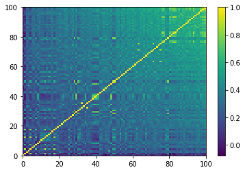
The equivalent correlation matrix.
Note that this representation is the one obtained after re-ordering using the *canonical_repr* function.
Below, an implementation of the GAN in TF 2.0 with the Keras API.
BUFFER_SIZE = corrs.shape[0]
BATCH_SIZE = 256
# Batch and shuffle the data
train_dataset = (tf
                 .data.Dataset.from_tensor_slices(corrs)
                 .shuffle(BUFFER_SIZE)
                 .batch(BATCH_SIZE))
def make_generator_model():
    model = tf.keras.Sequential()
    model.add(layers.Dense(512, use_bias=False, input_shape=(100,)))
    model.add(layers.BatchNormalization())
    model.add(layers.LeakyReLU())

    model.add(layers.Dense(1024, use_bias=False))
    model.add(layers.BatchNormalization())
    model.add(layers.LeakyReLU())

    model.add(layers.Dense(2048, use_bias=False))
    model.add(layers.BatchNormalization())
    model.add(layers.LeakyReLU())

    model.add(layers.Dense(int(n * (n - 1) / 2),
                           use_bias=False,
                           activation='tanh'))

    return model
generator = make_generator_model()

noise = tf.random.normal([1, 100])
generated_image = generator(noise, training=False)

plt.plot(generated_image[0, :])
plt.show()
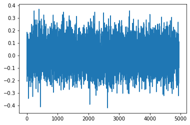
Before any training of the generator: noise in, noise out.
def make_discriminator_model():
    model = tf.keras.Sequential()
    model.add(layers.Dense(1024, input_shape=[int(n * (n - 1) / 2)]))
    model.add(layers.LeakyReLU())
    model.add(layers.Dropout(0.3))

    model.add(layers.Dense(512))
    model.add(layers.LeakyReLU())
    model.add(layers.Dropout(0.3))

    model.add(layers.Dense(128))
    model.add(layers.LeakyReLU())
    model.add(layers.Dropout(0.3))

    model.add(layers.Dense(64))
    model.add(layers.LeakyReLU())
    model.add(layers.Dropout(0.3))

    model.add(layers.Flatten())
    model.add(layers.Dense(1))

    return model
discriminator = make_discriminator_model()
decision = discriminator(generated_image)
print(decision)
tf.Tensor([[0.0345522]], shape=(1, 1), dtype=float32)
# This method returns a helper function to compute cross entropy loss
cross_entropy = tf.keras.losses.BinaryCrossentropy(from_logits=True)
def discriminator_loss(real_output, fake_output):
    real_loss = cross_entropy(tf.ones_like(real_output),
                              real_output)
    fake_loss = cross_entropy(tf.zeros_like(fake_output),
                              fake_output)
    total_loss = real_loss + fake_loss
    return total_loss
def generator_loss(fake_output):
    return cross_entropy(tf.ones_like(fake_output),
                         fake_output)
generator_optimizer = tf.keras.optimizers.Adam(1e-4)
discriminator_optimizer = tf.keras.optimizers.Adam(1e-4)
EPOCHS = 10000
noise_dim = 100
num_examples_to_generate = 16

# We will reuse this seed overtime (so it's easier)
# to visualize progress in the animated GIF)
seed = tf.random.normal([num_examples_to_generate, noise_dim])
# Notice the use of `tf.function`
# This annotation causes the function to be "compiled".
@tf.function
def train_step(images):
    noise = tf.random.normal([BATCH_SIZE, noise_dim])

    with tf.GradientTape() as gen_tape, tf.GradientTape() as disc_tape:
        generated_images = generator(noise, training=True)

        real_output = discriminator(images, training=True)
        fake_output = discriminator(generated_images, training=True)

        gen_loss = generator_loss(fake_output)
        disc_loss = discriminator_loss(real_output, fake_output)

    gradients_of_generator = gen_tape.gradient(
        gen_loss, generator.trainable_variables)
    gradients_of_discriminator = disc_tape.gradient(
        disc_loss, discriminator.trainable_variables)

    generator_optimizer.apply_gradients(
        zip(gradients_of_generator, generator.trainable_variables))
    discriminator_optimizer.apply_gradients(
        zip(gradients_of_discriminator, discriminator.trainable_variables))
def train(dataset, epochs):
    for epoch in range(epochs):
        start = time.time()

        for image_batch in dataset:
            train_step(image_batch)

        # Produce images for the GIF as we go
        display.clear_output(wait=True)
        generate_and_save_images(generator,
                                 epoch + 1,
                                 seed)

        print ('Time for epoch {} is {} sec'.format(
            epoch + 1, time.time() - start))

    # Generate after the final epoch
    display.clear_output(wait=True)
    generate_and_save_images(generator,
                             epochs,
                             seed)
def generate_and_save_images(model, epoch, test_input):
    # Notice `training` is set to False.
    # This is so all layers run in inference mode (batchnorm).
    predictions = model(test_input, training=False)

    fig = plt.figure(figsize=(16, 16))

    for i in range(predictions.shape[0]):
        prediction = predictions[i, :]
        corr = np.ones((n, n))
        corr[a, b] = prediction
        corr[b, a] = prediction
        plt.subplot(4, 4, i + 1)
        plt.imshow(corr)
        plt.axis('off')

    plt.savefig('v3_image_at_epoch_{:04d}.png'.format(epoch))
    plt.show()
%%time
train(train_dataset, EPOCHS)
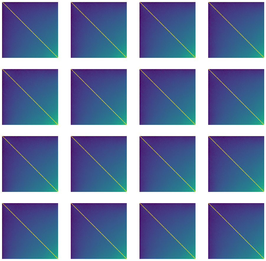
Time for epoch 10000 is 11.296852111816406 sec
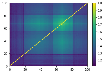
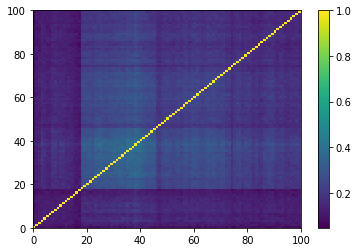
We generate one correlation matrix from the GAN (top the flatten representation, bottom the square matrix representation):
noise = tf.random.normal([1, 100])
generated_image = generator(noise, training=False)

plt.plot(generated_image[0, :])
plt.show()

c = np.ones((n, n))
c[a, b] = generated_image[0, :]
c[b, a] = generated_image[0, :]

plt.pcolormesh(c)
plt.colorbar()
plt.show()

(Left) Correlation coefficients generated by the GAN; (Right) Empirical correlation coefficients estimated from stocks' returns.
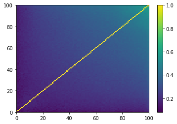
(Left) Correlation matrix generated by the GAN; (Right) Empirical correlation matrix estimated from stocks' returns.
Remark. The correlations generated seem too smooth with respect to the real data. To explore further the discrepancy between real and generated data, let’s look at the stylized properties of financial correlations below.
Let’s first generate, using the GAN, nb_samples = 100 correlation matrices. We will compare with another sample of 100 empirical correlation matrices estimated from real historical returns.
nb_samples = 100

generated_correls = []
for i in range(nb_samples):
    noise = tf.random.normal([1, 100])
    generated_image = generator(noise, training=False)
    correls = np.array(generated_image[0, :])
    generated_correls.extend(list(correls))

empirical_correls = []
for i in range(len(corrs[:min(nb_samples, len(corrs)), :])):
    empirical = corrs[i, :]
    empirical_correls.extend(list(empirical))
len(generated_correls), len(empirical_correls)
(495000, 495000)
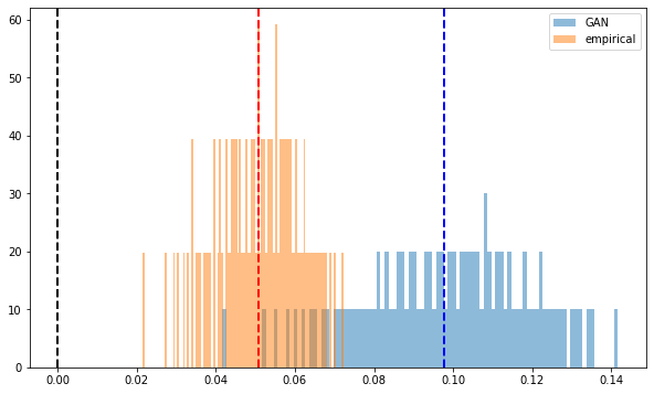
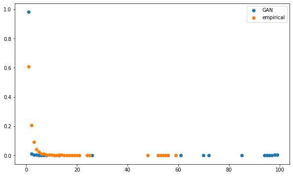
Let’s look at the distribution of these correlation coefficients:
plt.hist(generated_correls, bins=100, alpha=0.5,
         density=True, label='GAN correlations')
plt.hist(empirical_correls, bins=100, alpha=0.5,
         density=True, label='empirical correlations')
plt.axvline(x=np.mean(generated_correls),
            color='b', linestyle='dashed', linewidth=2)
plt.axvline(x=np.mean(empirical_correls),
            color='r', linestyle='dashed', linewidth=2)
plt.legend()
plt.show()

plt.hist(generated_correls, bins=100, alpha=0.5,
         density=True, log=True, label='GAN correlations')
plt.hist(empirical_correls, bins=100, alpha=0.5,
         density=True, log=True, label='empirical correlations')
plt.axvline(x=np.mean(generated_correls),
            color='b', linestyle='dashed', linewidth=2)
plt.axvline(x=np.mean(empirical_correls),
            color='r', linestyle='dashed', linewidth=2)
plt.legend()
plt.show()
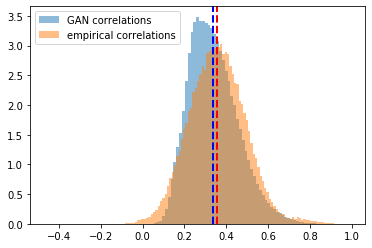
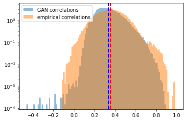
First, we notice that the mean of the two distributions is quite close (at around 0.35). The GAN has effectively learnt the distribution mean! However, the GAN fails at learning the right tail (a few coefficients are very high, close to 0.98), and fails to capture the non-existence of a left tail (correlations between stocks are usually not negative, and when they are, small in absolute value).
Then, let’s look at the distribution of their eigenvalues:
nb_samples = 100

generated_corr_mats = []
for i in range(nb_samples):
    noise = tf.random.normal([1, 100])
    generated_image = generator(noise, training=False)
    correls = np.array(generated_image[0, :])
    corr_mat = np.ones((n, n))
    corr_mat[a, b] = correls
    corr_mat[b, a] = correls
    generated_corr_mats.append(corr_mat)

empirical_corr_mats = []
for i in range(len(corrs[:min(nb_samples, len(corrs)), :])):
    empirical = corrs[i, :]
    corr_mat = np.ones((n, n))
    corr_mat[a, b] = empirical
    corr_mat[b, a] = empirical
    empirical_corr_mats.append(corr_mat)
def compute_eigenvals(correls):
    eigenvalues = []
    for corr in correls:
        eigenvals, eigenvecs = np.linalg.eig(corr)
        eigenvalues.append(sorted(eigenvals, reverse=True))

    return eigenvalues

sample_mean_empirical_eigenvals = np.mean(
    compute_eigenvals(empirical_corr_mats), axis=0)
sample_mean_gan_eigenvals = np.mean(
    compute_eigenvals(generated_corr_mats), axis=0)
plt.figure(figsize=(10, 6))
plt.hist(sample_mean_gan_eigenvals, bins=n,
         density=True, alpha=0.5, label='GAN')
plt.hist(sample_mean_empirical_eigenvals, bins=n,
         density=True, alpha=0.5, label='empirical')
plt.legend()
plt.show()
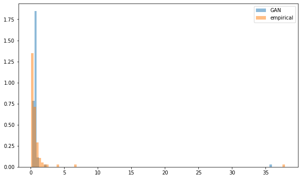
Both have a very large first eigenvalue (capturing the market mode / the base correlation), but unlike the empirical case, the GAN-generated matrices don’t have a couple of large eigenvalues far apart the bulk of eigenvalues. Usually, these large eigenvalues correspond to the main factors (drivers of returns), that is for stocks from the same economic region, the industrial sectors. It seems that the GAN-generated matrices exhibit only one large eigenvalue outside the bulk, aside from the “market” eigenvalue. Put another way, these matrices should contain only one cluster.
Let’s verify that by re-ordering the correlation matrices using a hierarchical clustering algorithm later.
Concerning the Perron-Frobenius property (first eigenvector has positive entries):
def compute_pf_vec(correls):
    pf_vectors = []
    for corr in correls:
        eigenvals, eigenvecs = np.linalg.eig(corr)
        pf_vector = eigenvecs[:, np.argmax(eigenvals)]
        if len(pf_vector[pf_vector < 0]) > len(pf_vector[pf_vector > 0]):
            pf_vector = -pf_vector
        pf_vectors.append(pf_vector)

    return pf_vectors

mean_empirical_pf = np.mean(
    compute_pf_vec(empirical_corr_mats), axis=0)
mean_gan_pf = np.mean(
    compute_pf_vec(generated_corr_mats), axis=0)
plt.figure(figsize=(10, 6))
plt.hist(mean_gan_pf, bins=n, density=True,
         alpha=0.5, label='GAN')
plt.hist(mean_empirical_pf, bins=n, density=True,
         alpha=0.5, label='empirical')
plt.axvline(x=0,
            color='k', linestyle='dashed', linewidth=2)
plt.axvline(x=np.mean(mean_gan_pf),
            color='b', linestyle='dashed', linewidth=2)
plt.axvline(x=np.mean(mean_empirical_pf),
            color='r', linestyle='dashed', linewidth=2)
plt.legend()
plt.show()
Perron-Frobenius property (first eigenvector has positive entries) is verified, but the distributions don't closely match.
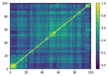
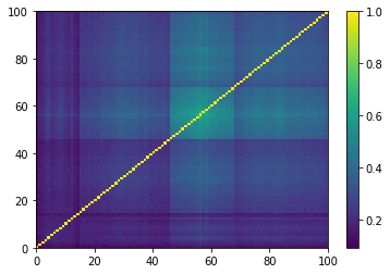
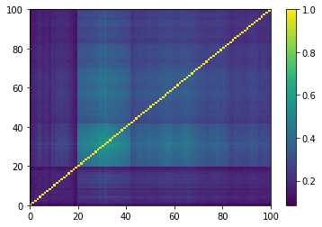
Concerning the hierarchical clustering property:
for idx, corr in enumerate(empirical_corr_mats):
    dist = 1 - corr
    Z = fastcluster.linkage(dist[a, b], method='ward')
    permutation = hierarchy.leaves_list(
        hierarchy.optimal_leaf_ordering(Z, dist[a, b]))
    prows = corr[permutation, :]
    ordered_corr = prows[:, permutation]

    plt.pcolormesh(ordered_corr)
    plt.colorbar()
    plt.show()

    if idx > 5:
        break
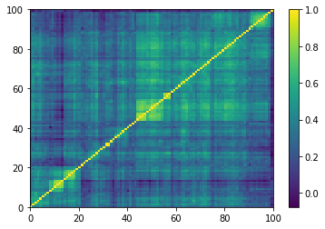
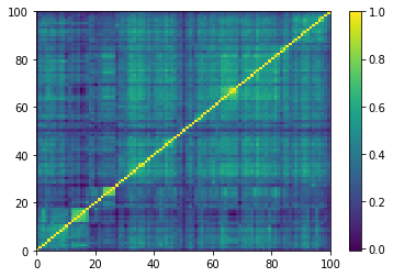

Empirical correlation matrices do verify this property, and the clusters correspond to industrial sectors.
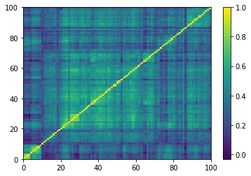
for idx, corr in enumerate(generated_corr_mats):
    dist = 1 - corr
    Z = fastcluster.linkage(dist[a, b], method='ward')
    permutation = hierarchy.leaves_list(
        hierarchy.optimal_leaf_ordering(Z, dist[a, b]))
    prows = corr[permutation, :]
    ordered_corr = prows[:, permutation]

    plt.pcolormesh(ordered_corr)
    plt.colorbar()
    plt.show()

    if idx > 5:
        break

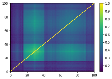
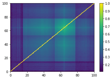
As expected by the study of eigenvalues, the GAN-generated matrices do not really contain clusters, but maybe a broad one that is not very distant (uncorrelated) to the rest. This should mean that a few “artificial” stocks are strongly connected to most of the other stocks. And, we can read also from these matrices, that many of the “artificial” stocks are not connected to others but to this central stocks.
We can verify this claim with a quick network study.
Let’s compute the minimum spanning tree (MST) (cf. this review pointing to a vast literature of networks applications in financial markets). From this MST, let’s extract an important summary statistics: the distribution of the vertices’ degrees (k(i) = the number of vertices connected to the given vertex i; d(k) = the normalised number of vertices having degree k).
For empirical correlation matrices, this distribution should roughly follow a power law (linear relationship between degree and frequency in log-log plot).
def compute_degree_counts(correls):
    all_counts = []
    for corr in correls:
        dist = (1 - corr) / 2
        G = nx.from_numpy_matrix(dist)
        mst = nx.minimum_spanning_tree(G)

        degrees = {i: 0 for i in range(len(corr))}
        for edge in mst.edges:
            degrees[edge[0]] += 1
            degrees[edge[1]] += 1
        degrees = pd.Series(degrees).sort_values(ascending=False)
        cur_counts = degrees.value_counts()
        counts = np.zeros(len(corr))
        for i in range(len(corr)):
            if i in cur_counts:
                counts[i] = cur_counts[i]

        all_counts.append(counts / (len(corr) - 1))

    return all_counts
mean_gan_counts = np.mean(
    compute_degree_counts(generated_corr_mats), axis=0)
mean_gan_counts = (pd
                   .Series(mean_gan_counts)
                   .replace(0, np.nan))

mean_empirical_counts = np.mean(
    compute_degree_counts(empirical_corr_mats), axis=0)
mean_empirical_counts = (pd
                         .Series(mean_empirical_counts)
                         .replace(0, np.nan))
plt.figure(figsize=(10, 6))
plt.scatter(mean_gan_counts.index,
            mean_gan_counts,
            label='GAN')
plt.scatter(mean_empirical_counts.index,
            mean_empirical_counts,
            label='empirical')
plt.legend()
plt.show()
plt.figure(figsize=(10, 6))
plt.scatter(np.log10(mean_gan_counts.index),
            np.log10(mean_gan_counts),
            label='GAN')
plt.scatter(np.log10(mean_empirical_counts.index),
            np.log10(mean_empirical_counts),
            label='empirical')
plt.legend()
plt.show()
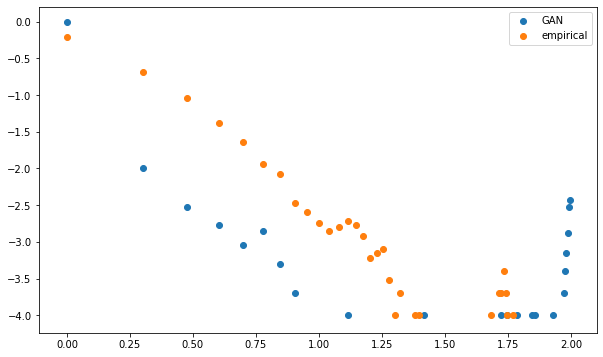
Again, the distributions do not closely match.
It confirms what we hypothesised with the visual representation: A few nodes are strongly connected to the rest, and many nodes have few connections. In the case of GAN-generated matrices/networks, the number of leaves (degree one, i.e. only one connection) is abnormally high; the ‘too low’ number of ‘average’ degrees (the linear log-log relationship) hints at a lack of hierarchical structure (communities). This power-law-like feature is characteristic of complex systems, and has been described in the context of financial correlations many times since 1999, for a variety of asset classes.
Conclusion: Still some work to do. A vanilla GAN was not able to capture precisely the empirical distribution of these financial correlation matrices. What’s next? More training samples (only ~9000 in this experiment)? More epochs (10,000 here, but seems to have reached an equilibrium)? A different representation for the matrices? A more relevant architecture for the discriminator and/or generator?