TF 2.0 DCGAN for 100x100 financial correlation matrices
TF 2.0 DCGAN for 100x100 financial correlation matrices
We concluded the previous experiment with
[…] A vanilla GAN was not able to capture precisely the empirical distribution of these financial correlation matrices. What’s next? More training samples (only ~9000 in this experiment)? More epochs (10,000 here, but seems to have reached an equilibrium)? A different representation for the matrices? A more relevant architecture for the discriminator and/or generator?
In this blog post, we will keep the same training sample, but we will use a different GAN architecture, namely DCGAN, and a different representation for the correlation matrices, a re-ordering using a deterministic hierarchical clustering algorithm.
TL;DR We show in this blog that we are able to recover the main stylized facts of financial correlation matrices using a DCGAN. The DCGAN used is trained on ~ 9000 empirical financial correlation matrices estimated on the returns of 100 randomly selected stocks members of the S&P 500 index.
Correlation matrices were re-ordered using a deterministic hierarchical clustering algorithm. This re-ordering is used for two reasons:
-
alleviate the problems mentioned in the blog “Permutation invariance in Neural networks“, i.e. n! matrices are equivalent but outputs of a standard neural network can be different, thus making the training on realistically sized samples difficult;
-
DCGAN is known to learn a hierarchy of representations from object parts to scenes in natural images; in this context, it can be useful to capture the hierarchical nature of financial correlations.
We are able to obtain reasonable results with relatively few epochs (~ 2000+).
(Left) Empirical correlation matrix estimated on stocks returns; (Right) GAN-generated correlation matrix.
import tensorflow as tf
tf.__version__
'2.0.0-rc1'
%matplotlib inline

import os
import time
import glob
import imageio
import matplotlib.pyplot as plt
import pandas as pd
import numpy as np
import fastcluster
import networkx as nx
from scipy.cluster import hierarchy
import PIL
from tensorflow.keras import layers
from statsmodels.stats.correlation_tools import corr_nearest

from IPython import display
Loading the training set…
n = 100
a, b = np.triu_indices(n, k=1)

corrs = []
for r, d, files in os.walk('sorted_corrs/'):
    for file in files:
        if 'corr_emp_{}d_batch_'.format(n) in file:
            flat_corr = pd.read_hdf('sorted_corrs/{}'.format(file))
            corr = np.ones((n, n))
            corr[a, b] = flat_corr
            corr[b, a] = flat_corr
            corrs.append(corr)
corrs = (np
         .array(corrs)
         .reshape(len(corrs), n, n, 1)
         .astype('float32'))
corrs.shape
(9196, 100, 100, 1)
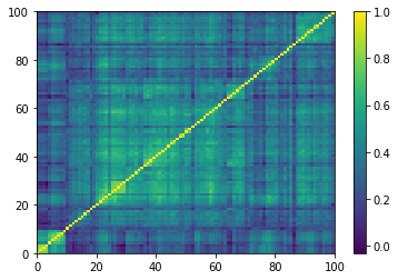
plt.pcolormesh(corrs[0, :, :, 0])
plt.colorbar()
plt.show()

One of the 9196 empirical 100x100 correlation matrices that consist in the training set for the DCGAN. Note that the rows and columns were re-ordered using a deterministic hierarchical clustering algorithm. This representation goes hand in hand with the architecture of the DCGAN, known to learn a hierarchy of representations from object parts to scenes in natural images.
BUFFER_SIZE = corrs.shape[0]
BATCH_SIZE = 256
# Batch and shuffle the data
train_dataset = (tf
                 .data.Dataset.from_tensor_slices(corrs)
                 .shuffle(BUFFER_SIZE)
                 .batch(BATCH_SIZE))
The DCGAN generator:
def make_generator_model():
    model = tf.keras.Sequential()
    model.add(layers.Dense(25 * 25 * 256,
                           use_bias=False,
                           input_shape=(100,)))
    model.add(layers.BatchNormalization())
    model.add(layers.LeakyReLU())

    model.add(layers.Reshape((25, 25, 256)))
    assert model.output_shape == (None, 25, 25, 256)

    model.add(layers.Conv2DTranspose(128, (5, 5),
                                     strides=(1, 1),
                                     padding='same',
                                     use_bias=False))
    assert model.output_shape == (None, 25, 25, 128)
    model.add(layers.BatchNormalization())
    model.add(layers.LeakyReLU())

    model.add(layers.Conv2DTranspose(64, (5, 5),
                                     strides=(2, 2),
                                     padding='same',
                                     use_bias=False))
    assert model.output_shape == (None, 50, 50, 64)
    model.add(layers.BatchNormalization())
    model.add(layers.LeakyReLU())

    model.add(layers.Conv2DTranspose(1, (5, 5),
                                     strides=(2, 2),
                                     padding='same',
                                     use_bias=False,
                                     activation='tanh'))
    assert model.output_shape == (None, 100, 100, 1)

    return model
generator = make_generator_model()

noise = tf.random.normal([1, 100])
generated_image = generator(noise, training=False)

plt.pcolormesh(generated_image[0, :, :, 0])
plt.colorbar()
plt.show()
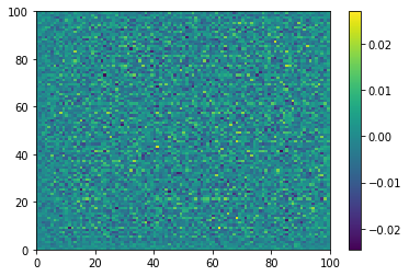
Before any training of the generator: noise in, noise out.
The DCGAN discriminator:
def make_discriminator_model():
    model = tf.keras.Sequential()
    model.add(layers.Conv2D(64, (5, 5),
                            strides=(2, 2),
                            padding='same',
                            input_shape=[100, 100, 1]))
    model.add(layers.LeakyReLU())
    model.add(layers.Dropout(0.3))

    model.add(layers.Conv2D(128, (5, 5),
                            strides=(2, 2),
                            padding='same'))
    model.add(layers.LeakyReLU())
    model.add(layers.Dropout(0.3))

    model.add(layers.Flatten())
    model.add(layers.Dense(1))

    return model
discriminator = make_discriminator_model()
decision = discriminator(generated_image)
print(decision)
tf.Tensor([[2.2654163e-05]], shape=(1, 1), dtype=float32)
# This method returns a helper function to compute cross entropy loss
cross_entropy = tf.keras.losses.BinaryCrossentropy(from_logits=True)
def discriminator_loss(real_output, fake_output):
    real_loss = cross_entropy(tf.ones_like(real_output),
                              real_output)
    fake_loss = cross_entropy(tf.zeros_like(fake_output),
                              fake_output)
    total_loss = real_loss + fake_loss
    return total_loss
def generator_loss(fake_output):
    return cross_entropy(tf.ones_like(fake_output),
                         fake_output)
generator_optimizer = tf.keras.optimizers.Adam(1e-4)
discriminator_optimizer = tf.keras.optimizers.Adam(1e-4)
EPOCHS = 10000
noise_dim = 100
num_examples_to_generate = 16

# We will reuse this seed overtime (so it's easier)
# to visualize progress in the animated GIF)
seed = tf.random.normal([num_examples_to_generate, noise_dim])
# Notice the use of `tf.function`
# This annotation causes the function to be "compiled".
@tf.function
def train_step(images):
    noise = tf.random.normal([BATCH_SIZE, noise_dim])

    with tf.GradientTape() as gen_tape, tf.GradientTape() as disc_tape:
        generated_images = generator(noise, training=True)

        real_output = discriminator(images, training=True)
        fake_output = discriminator(generated_images, training=True)

        gen_loss = generator_loss(fake_output)
        disc_loss = discriminator_loss(real_output, fake_output)

    gradients_of_generator = gen_tape.gradient(
        gen_loss, generator.trainable_variables)
    gradients_of_discriminator = disc_tape.gradient(
        disc_loss, discriminator.trainable_variables)

    generator_optimizer.apply_gradients(
        zip(gradients_of_generator, generator.trainable_variables))
    discriminator_optimizer.apply_gradients(
        zip(gradients_of_discriminator, discriminator.trainable_variables))
def train(dataset, epochs):
    for epoch in range(epochs):
        start = time.time()

        for image_batch in dataset:
            train_step(image_batch)

        # Produce images for the GIF as we go
        display.clear_output(wait=True)
        generate_and_save_images(generator,
                                 epoch + 1,
                                 seed)

        print ('Time for epoch {} is {} sec'.format(
            epoch + 1, time.time() - start))

    # Generate after the final epoch
    display.clear_output(wait=True)
    generate_and_save_images(generator,
                             epochs,
                             seed)
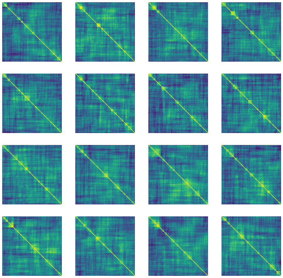
def generate_and_save_images(model, epoch, test_input):
    # Notice `training` is set to False.
    # This is so all layers run in inference mode (batchnorm).
    predictions = model(test_input, training=False)

    fig = plt.figure(figsize=(16, 16))

    for i in range(predictions.shape[0]):
        plt.subplot(4, 4, i + 1)
        plt.imshow(predictions[i, :, :, 0])
        plt.axis('off')

    plt.savefig('v2_image/v2_image_at_epoch_{:04d}.png'.format(epoch))
    plt.show()
%%time
train(train_dataset, EPOCHS)
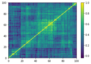
"Correlation" matrices generated using DCGAN after epoch 3517.
Time for epoch 3517 is 508.3090147972107 sec
noise = tf.random.normal([1, 100])
generated_image = generator(noise, training=False)

plt.pcolormesh(generated_image[0, :, :, 0])
plt.colorbar()
plt.show()

From a random vector to a random "correlation" matrix.
The matrices generated are not strictly speaking correlation matrices: Their diagonal is not exactly equal to 1; they are not exactly symmetric, and one can find some small negative eigenvalues.
gan_correls = np.array(generated_image[0, :, :, 0])
(pd
 .Series([gan_correls[i, i] for i in range(len(gan_correls))],
         index=[i + 1 for i in range(len(gan_correls))])
 .plot())
(pd
 .Series([gan_correls[i, i] for i in range(5, len(gan_correls)-5)],
         index=[i + 1 for i in range(5, len(gan_correls)-5)])
 .plot())
(pd
 .Series([1] * n, index=list(range(1, n + 1)))
 .plot())
plt.show()
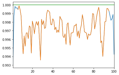
A proper correlation matrix should have unit diagonal; The matrices produced by DCGAN have diagonals close, but not strictly equal, to 1.
We can fix this problem by projecting on the nearest correlation matrix using Higham’s alternating projections method.
nb_samples = 500

generated_correls = []
for i in range(nb_samples):
    noise = tf.random.normal([1, 100])
    generated_image = generator(noise, training=False)
    correls = np.array(generated_image[0,:,:,0])
    generated_correls.extend(list(correls[a, b]))

empirical_correls = []
for i in range(len(corrs[:min(nb_samples, len(corrs)), :, :, :])):
    empirical = corrs[i, :, :, 0]
    empirical_correls.extend(list(empirical[a, b]))
len(generated_correls), len(empirical_correls)
(2475000, 2475000)
plt.hist(generated_correls, bins=100, alpha=0.5,
         density=True, label='DCGAN correlations')
plt.hist(empirical_correls, bins=100, alpha=0.5,
         density=True, label='empirical correlations')
plt.axvline(x=np.mean(generated_correls),
            color='b', linestyle='dashed', linewidth=2)
plt.axvline(x=np.mean(empirical_correls),
            color='r', linestyle='dashed', linewidth=2)
plt.legend()
plt.show()

plt.hist(generated_correls, bins=100, alpha=0.5,
         density=True, log=True, label='DCGAN correlations')
plt.hist(empirical_correls, bins=100, alpha=0.5,
         density=True, log=True, label='empirical correlations')
plt.axvline(x=np.mean(generated_correls),
            color='b', linestyle='dashed', linewidth=2)
plt.axvline(x=np.mean(empirical_correls),
            color='r', linestyle='dashed', linewidth=2)
plt.legend()
plt.show()
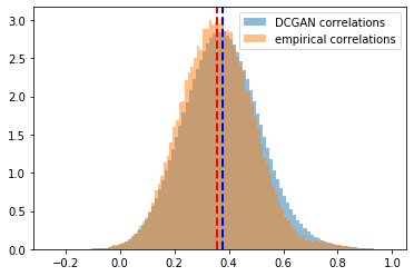
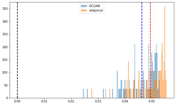
Distribution of the correlation coefficients. Mean of the empirical correlations and mean of the generated correlations are approximately equal (~0.37), their standard deviation too (~0.13). Some discrepancies around the tails.
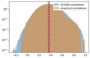
Log-distribution to highlight the discrepancies in the tails of the distributions.
corr_nearest implements the projection to the nearest correlation so that matrices are positive semidefinite, and therefore, with symmetry and unit diagonal, proper correlation matrices.
nb_samples = 500

generated_corr_mats = []
for i in range(nb_samples):
    print(i + 1, "/", nb_samples)

    noise = tf.random.normal([1, 100])
    generated_image = generator(noise, training=False)
    correls = np.array(generated_image[0,:,:,0])
    # set diag to 1
    np.fill_diagonal(correls, 1)
    # symmetrize
    correls[b, a] = correls[a, b]
    # nearest corr
    nearest_correls = corr_nearest(correls)
    # set diag to 1
    np.fill_diagonal(nearest_correls, 1)
    # symmetrize
    nearest_correls[b, a] = nearest_correls[a, b]

    generated_corr_mats.append(nearest_correls)

empirical_corr_mats = []
for i in range(len(corrs[:min(nb_samples, len(corrs)), :, :, :])):
    empirical = corrs[i, :, :, 0]
    empirical_corr_mats.append(empirical)
The distribution of eigenvalues closely match: They both exhibit a very large first eigenvalue (representing the market), and a few eigenvalues outside of the best fit Marchenko–Pastur distribution support (corresponding to industrial sectors).
def compute_eigenvals(correls):
    eigenvalues = []
    for corr in correls:
        eigenvals, eigenvecs = np.linalg.eig(corr)
        eigenvalues.append(sorted(eigenvals, reverse=True))

    return eigenvalues

sample_mean_empirical_eigenvals = np.mean(
    compute_eigenvals(empirical_corr_mats), axis=0)
sample_mean_dcgan_eigenvals = np.mean(
    compute_eigenvals(generated_corr_mats), axis=0)
plt.figure(figsize=(10, 6))
plt.hist(sample_mean_dcgan_eigenvals, bins=n,
         density=True, alpha=0.5, label='DCGAN')
plt.hist(sample_mean_empirical_eigenvals, bins=n,
         density=True, alpha=0.5, label='empirical')
plt.legend()
plt.show()
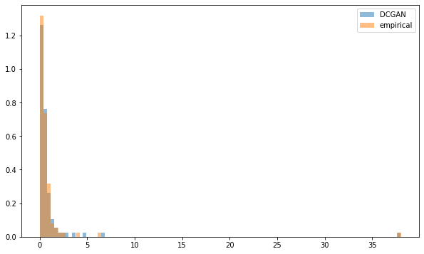
The distribution of eigenvalues closely match.
def compute_pf_vec(correls):
    pf_vectors = []
    for corr in correls:
        eigenvals, eigenvecs = np.linalg.eig(corr)
        pf_vector = eigenvecs[:, np.argmax(eigenvals)]
        if len(pf_vector[pf_vector < 0]) > len(pf_vector[pf_vector > 0]):
            pf_vector = -pf_vector
        pf_vectors.append(pf_vector)

    return pf_vectors

mean_empirical_pf = np.mean(
    compute_pf_vec(empirical_corr_mats), axis=0)
mean_dcgan_pf = np.mean(
    compute_pf_vec(generated_corr_mats), axis=0)
plt.figure(figsize=(10, 6))
plt.hist(mean_dcgan_pf, bins=n, density=True,
         alpha=0.5, label='DCGAN')
plt.hist(mean_empirical_pf, bins=n, density=True,
         alpha=0.5, label='empirical')
plt.axvline(x=0,
            color='k', linestyle='dashed', linewidth=2)
plt.axvline(x=np.mean(mean_dcgan_pf),
            color='b', linestyle='dashed', linewidth=2)
plt.axvline(x=np.mean(mean_empirical_pf),
            color='r', linestyle='dashed', linewidth=2)
plt.legend()
plt.show()
Distribution of the first eigenvector entries. All positive.
Empirical and synthetic distributions are matching closely.
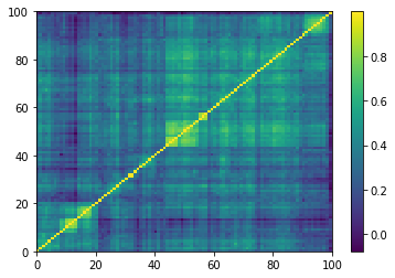
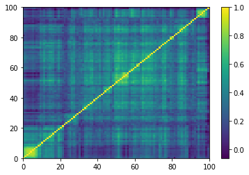
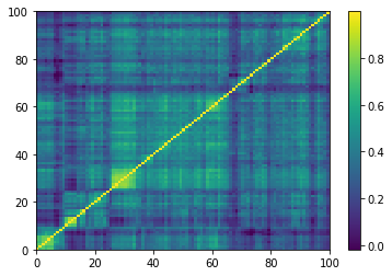
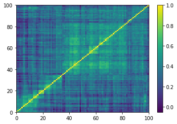
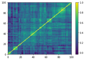
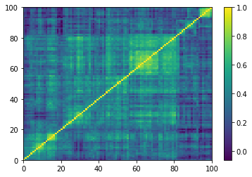
Displaying a few empirical correlation matrices:
for idx, corr in enumerate(empirical_corr_mats):
    dist = 1 - corr
    Z = fastcluster.linkage(dist[a, b], method='ward')
    permutation = hierarchy.leaves_list(
        hierarchy.optimal_leaf_ordering(Z, dist[a, b]))
    prows = corr[permutation, :]
    ordered_corr = prows[:, permutation]

    plt.pcolormesh(ordered_corr)
    plt.colorbar()
    plt.show()

    if idx > 5:
        break
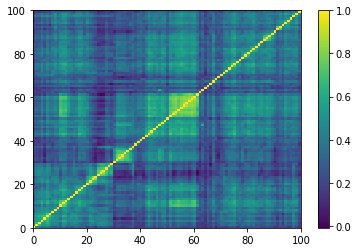
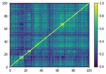
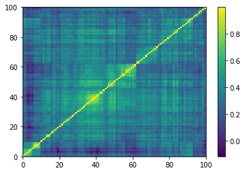
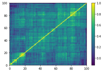
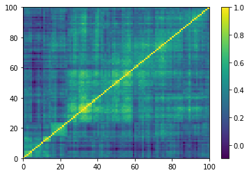
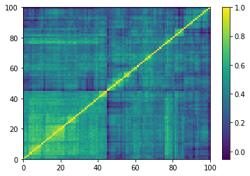
Displaying a few GAN-generated (with projection to the nearest correlation post-processing) correlation matrices:
for idx, corr in enumerate(generated_corr_mats):
    # cheat: set diagonal to 1
    np.fill_diagonal(corr, 1)
    dist = 1 - corr
    Z = fastcluster.linkage(dist[a, b], method='ward')
    permutation = hierarchy.leaves_list(
        hierarchy.optimal_leaf_ordering(Z, dist[a, b]))
    prows = corr[permutation, :]
    ordered_corr = prows[:, permutation]

    plt.pcolormesh(ordered_corr)
    plt.colorbar()
    plt.show()

    if idx > 5:
        break
Computing the Minimum Spanning Tree, and the associated distribution of node degrees:
def compute_degree_counts(correls):
    all_counts = []
    for corr in correls:
        dist = (1 - corr) / 2
        G = nx.from_numpy_matrix(dist)
        mst = nx.minimum_spanning_tree(G)

        degrees = {i: 0 for i in range(len(corr))}
        for edge in mst.edges:
            degrees[edge[0]] += 1
            degrees[edge[1]] += 1
        degrees = pd.Series(degrees).sort_values(ascending=False)
        cur_counts = degrees.value_counts()
        counts = np.zeros(len(corr))
        for i in range(len(corr)):
            if i in cur_counts:
                counts[i] = cur_counts[i]

        all_counts.append(counts / (len(corr) - 1))

    return all_counts
mean_dcgan_counts = np.mean(
    compute_degree_counts(generated_corr_mats), axis=0)
mean_dcgan_counts = (pd
                     .Series(mean_dcgan_counts)
                     .replace(0, np.nan))

mean_empirical_counts = np.mean(
    compute_degree_counts(empirical_corr_mats), axis=0)
mean_empirical_counts = (pd
                         .Series(mean_empirical_counts)
                         .replace(0, np.nan))
plt.figure(figsize=(10, 6))
plt.scatter(mean_dcgan_counts.index,
            mean_dcgan_counts,
            label='DCGAN')
plt.scatter(mean_empirical_counts.index,
            mean_empirical_counts,
            label='empirical')
plt.legend()
plt.show()
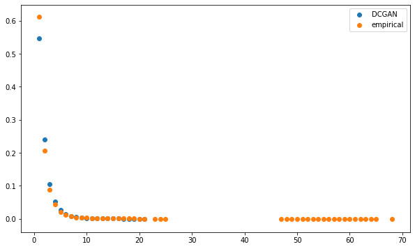
The distributions seem to be relatively close, but for the highest degrees which are only present for the empirical MSTs.
plt.figure(figsize=(10, 6))
plt.scatter(np.log10(mean_dcgan_counts.index),
            np.log10(mean_dcgan_counts),
            label='DCGAN')
plt.scatter(np.log10(mean_empirical_counts.index),
            np.log10(mean_empirical_counts),
            label='empirical')
plt.legend()
plt.show()
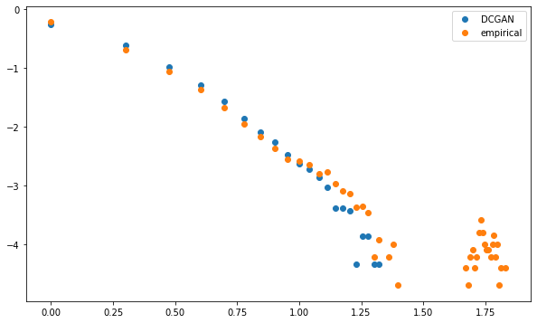
Both distributions are linear in the log-log plot (apparently following a power law with similar exponent), i.e. describing a scale-free network.
However, whereas MSTs computed on the GAN-generated correlation matrices exhibit this power law of node degrees without noticeable exceptions, empirical MSTs have "too many" nodes that are strongly connected. The GAN doesn't capture well this idiosyncrasy.
Conclusion: In this blog post, we show that some GANs are able to recover pretty well (at least part of) the distribution of empirical financial correlation matrices. A DCGAN trained on a good representation of the empirical financial correlation matrices, with a post-processing enforcing the mathematical constraints defining the elliptope, is able to generate correlation matrices that verify the well-known stylized facts. This generative model can be useful in many branches of quantitative finance.