[Paper] Summary of 'Explaining by Removing: A Unified Framework for Model Explanation'
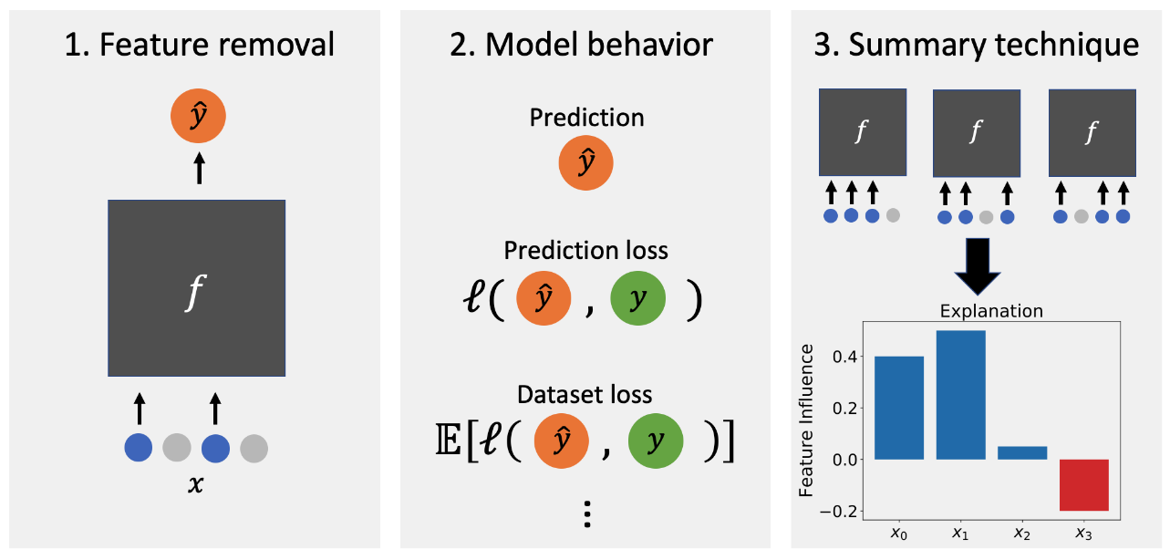 Illustration from Explaining by Removing: A Unified Framework for Model Explanation
[Paper] Summary of Explaining by Removing: A Unified Framework for Model Explanation
Paper: Explaining by Removing: A Unified Framework for Model Explanation by Ian Covert, Scott Lundberg, Su-In Lee.
Before this paper you had to understand 25+ seemingly very different feature importance methods, but now you just need to understand that you can combine 3 different choices of functions to cover the space of removal-based explanations.
caveat: It may still be beneficial to understand the peculiarities of each feature importance algorithm for computational complexity and efficient implementation reasons.
I predict this will be an influential paper with many citations to come… let’s see in 5 years!
Tbh, this summary doesn’t add much, if anything, to the paper. It’s more pointers for me in the future. If you have time on your hands, read the paper instead.
1. Introduction
Our framework is based on the observation that many methods can be understood as simulating feature removal to quantify each feature’s influenceon a model.
2. Background
The most active area of research in the field is local interpretability, which explains individual predictions, such as an individual patient diagnosis […]
in contrast, global interpretability explains the model’s behavior across the entire dataset
Both problems are usually addressed using feature attribution, where a score is assigned to explain each feature’s influence.
3. Removal-Based Explanations
One can find in the explainability literature 25 methods which are removal-based:
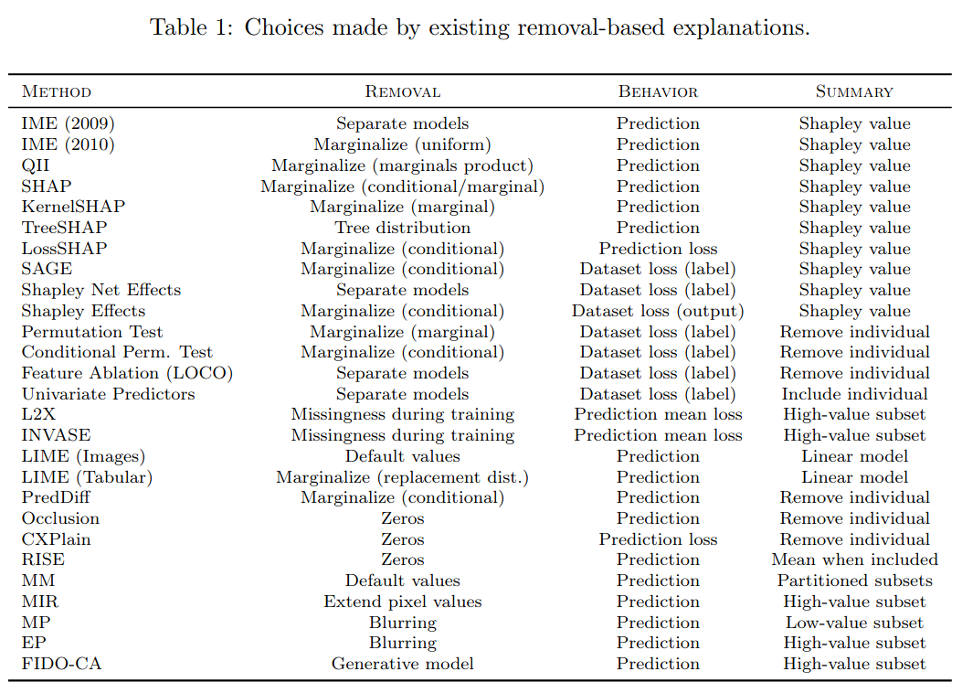 Illustration from Explaining by Removing: A Unified Framework for Model Explanation
These methods include many of the most widely used approaches (e.g. LIME and SHAP).
These methods are determined by three choices:
- feature removal
- model behavior
- summary technique
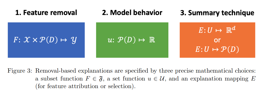 Illustration from Explaining by Removing: A Unified Framework for Model Explanation
4. Feature Removal
The first of the three choices.
A few formal definitions are needed.
Definition: A subset function is a mapping of the form $F : \mathcal{X} \times \mathcal{P}(D) \rightarrow \mathcal{Y}$ (that is, from the space of features $\mathcal{X}$ and a subset of the dimensions $\mathcal{P}(D)$ to the output domain $\mathcal{Y}$ of model $f : \mathcal{X} \rightarrow \mathcal{Y} \in \mathcal{f}$) that is invariant to the dimensions that are not in the specified subset. That is, $F(x, S) = F(x’, S)$ for all $(x, x’, S) \in \mathcal{X} \times \mathcal{X} \times \mathcal{P}(D)$ such that $x_S = x’_S$.
The space of all such subset functions is denoted $\mathfrak{F}$.
To be interesting to explain a model $f \in \mathcal{F}$, a subset function $F \in \mathfrak{F}$ must be an extension of $f$.
Definition: An extension of a model $f \in \mathcal{F}$ is a subset function $F \in \mathfrak{F}$ that agrees with $f$ in the presence of all features. That is, the model $f$ and its extension $F$ must satisfy $F(x, D) = f(x), \forall x \in \mathcal{X}$.
Then, removing features from a machine learning model can be understood and written in terms of the above formalism:
- Zero-ing features: $F(x, S) = f(x_S, 0)$
- Setting features to a default value $r$: $F(x, S) = f(x_S, r_{\overline{S}})$
- Sampling from a conditional generative model $\sim p_G(X_{\overline{S}} \vert X_S)$: $F(x, S) = f(x_S, \tilde{x}_{\overline{S}})$
- Marginalizing with condition: $F(x, S) = \mathbb{E}[ f(x) \vert X_S = x_S]$
- Marginalizing with marginal: $F(x, S) = \mathbb{E}[ f(x_S, X_{\overline{S}}) ]$
- …
We conclude that the first dimension of our framework amounts to choosing an extension $F \in \mathfrak{F}$ of the model $f \in \mathcal{F}$.
5. Explaining Different Model Behaviors
various choices of target quantities [can be observed] as different features are withheld from the model.
In fact, removal-based explanations need not be restricted to the ML context: any function that accommodates missing inputs can be explained via feature removal by examining either its output or some function of its output as groups of inputs are removed.
Many methods explain the model output or a simple function of the output, such as the log-odds ratio. Other methods take into account a measure of the model’s loss, for either an individual input or the entire dataset.
The model behavior can be captured by a function $u : \mathcal{P}(D) \rightarrow \mathbb{R}$.
For example, it can be
- at the prediction level (local explanations): Given an input $x \in \mathcal{X}$, study $F(x, S)$, that is how removed features are impacting a prediction higher or lower;
- at the prediction loss level (local explanations): Given an input $x$ and its true label $y$, study $-\ell(F(x, S), y)$, that is how some features are making the prediction more or less correct.
- the average prediction loss (local explanations): Given an input $x$ and the label’s conditional distribution $p(Y \vert X = x)$, study $-\mathbb{E}_{p(Y \vert X = x)}[ \ell(F(x, S), Y) ]$, that is how a certain set of features can correctly predict what could have occured on average. Can be useful with uncertain labels.
- dataset loss wrt label (global explanations): How much the model’s performance degrades when different features are removed, i.e. $-\mathbb{E}_{XY}[ \ell(F(X_S), Y) ]$
- dataset loss wrt output (global explanations): What are the features’ influence on the model output (rather than on the model performance), i.e. $-\mathbb{E}_X[ \ell(F(X_S), F(X)) ]$
These relationships show that explanations based on one set function are in some cases related to explanations based on another.
6. Summarizing Feature Influence
The third choice for removal-based explanations is how to summarize each feature’s influence on the model.
The set functions we used to represent a model’s dependence on different features (Section 5) are complicated mathematical objects that are difficult to communicate fully due to the exponential number of feature subsets and underlying feature interactions. Removal-based explanations confront this challenge by providing users with a concise summary of each feature’s influence.
We distinguish between two main types of summarization approaches: feature attributions and feature selections.
feature attributions $(a_1, a_2, \ldots, a_d) \in \mathbb{R}^d$: $E: \mathcal{U} \rightarrow \mathbb{R}^d$, where $\mathcal{U}$ is the set of all functions $u : \mathcal{P}(D) \rightarrow \mathbb{R}$.
feature selections: $E: \mathcal{U} \rightarrow \mathcal{P}(D)$
Both approaches provide users with simple summaries of a feature’s contribution to the set function.
Given this formalism, we can re-interpret many of the known methods (the removal-based ones):
- remove individual feature:
- include individual feature:
- mean when feature is included: $a_i = \mathbb{E}_{p(S \vert i \in S)}[ u(S) ]$
- Shapley value: $a_i = \phi_i(u)$
- low-value subset of features $S^{\star}$: $S^{\star} = argmin_S ~u(D \setminus S) + \lambda \lvert S \rvert$, with $\lambda > 0$
- high-value subset of features $S^{\star}$:
- $S^{\star} = argmin_S ~\lvert S \rvert$ s.t. $u(S) \geq t$, for a user-defined minimum value $t$
- $S^{\star} = argmax_S ~u(S)$ s.t. $\lvert S \rvert = k$, for a user-defined subset size $k$
- $S^{\star} = argmax_S ~u(S) - \lambda \lvert S \rvert$, with $\lambda > 0$
- partitioned subsets of features: $S^{\star} = argmax_S ~u(S) - \lambda u(D \setminus S) - \gamma \lvert S \rvert$, with $\lambda > 0, \gamma > 0$
These feature selection explanations are essentially coarse attributions that assign binary importance rather than a real number.
Though not generally viewed as a model explanation approach, global feature selection serves an identical purpose of identifying highly predictive features.
In fact, without making any simplifying assumptions about the model or data distribution, several techniques must examine all $2^d$ subsets of features.
Strategies that yield fast approximations include:
- attribution values that are the expectation of a random variable can be estimated using Monte Carlo approximations
- fit models to smaller sampled datasets, which means optimizing an approximate version of their objective function
- using a dynamic programming algorithm that exploits the structure of tree-based models
- solve continuous relaxations of their discrete optimization problems
- using a greedy optimization algorithm, iteratively removing groups of features
- learning separate explainer models
7. Game-Theoretic Explanations
The set function $u$ whose purpose is to explain the model $f$ can be interpreted as a cooperative game (defined the same way, as a function $u: \mathcal{P}(D) \rightarrow \mathbb{R}$) which describes the value achieved when sets of players $S \subseteq D$ participate in a game.
Player $i$’s marginal contribution is defined as .
The Shapley values $\phi_i(u) \in \mathbb{R}$ stem from this field, and are the unique allocations (vectors $z \in \mathbb{R}^d$ that represent payoffs proposed to each player in return for participating in the game) that satisfy the following properties:
- efficiency:
- symmetry:
- dummy:
- additivity:
- marginalism:
Shapley values:
Banzhaf values:
Banzhaf value $\psi_i(u)$ is the average marginal contribution of player $i$ in the cooperative game $u$.
The methods discussed thus far (Shapley value, Banzhaf value, removing individual players, including individual players) all satisfy the symmetry, dummy, additivity, and marginalism axioms. What makes the Shapley value unique among these methods is its efficiency axiom, which lets us view it as a distribution of the grand coalition’s value among the players (Dubey and Shapley, 1979).
These results show that the weighted least squares problem solved by LIME provides sufficient flexibility to express both the Shapley and Banzhaf values, as well as simpler quantities such as the marginal contributions from removing or including individual players. The LIME approach captures every feature attribution technique discussed so far
We have thus demonstrated that the LIME approach for summarizing feature influence not only has precedent in cooperative game theory, but is intimately connected to the other allocation strategies.
This suggests that the feature attributions generated by removal-based explanations should be viewed as additive decompositions of the underlying cooperative game $u$.
Definition: Given a cooperative game $u: \mathcal{P}(D) \rightarrow \mathbb{R}$, a coalition $S \subseteq D$, and an allocation $z = (z_1, z_2, \ldots, z_d) \in \mathbb{R}^d$, the excess of $S$ at $z$ is defined as $e(S, z) = u(S) - \sum_{i \in S} z_i$.
For cooperative games, excess measures the degree of unhappiness of players in the coalition: The higher the excess, the more the players feel cheated…
… and may refuse to take part in the game any longer. “We have no analogue for features refusing participation in ML, but the notion of excess is useful for understanding several removal-based explanation methods.” [pun of the authors]
Low-value and high-value subsets of features can be seen as finding the coalition whose complement has the lowest excess given an equal allocation, and finding the smallest possible coalition that achieves a sufficient level of excess given a zero allocation respectively.
Similar relations to the notion of excess can be derived for the feature selection methods discussed above. The paper describes them formally.
By reformulating the optimization problems solved by each method, we show that each feature selection summarization can be described as minimizing or maximizing excess given equal allocations for all players. In cooperative game theory, examining each coalition’s level of excess (or dissatisfaction) helps determine whether allocations will incentivize participation, but the same tool is used by removal-based explanations to find the most influential features for a model.
Finally, feature selection explanations provide only a coarse summary of each player’s value contribution, and their results depend on user-specified hyperparameters.
Each method’s summarization technique can be understood in terms of concepts from cooperative game theory:
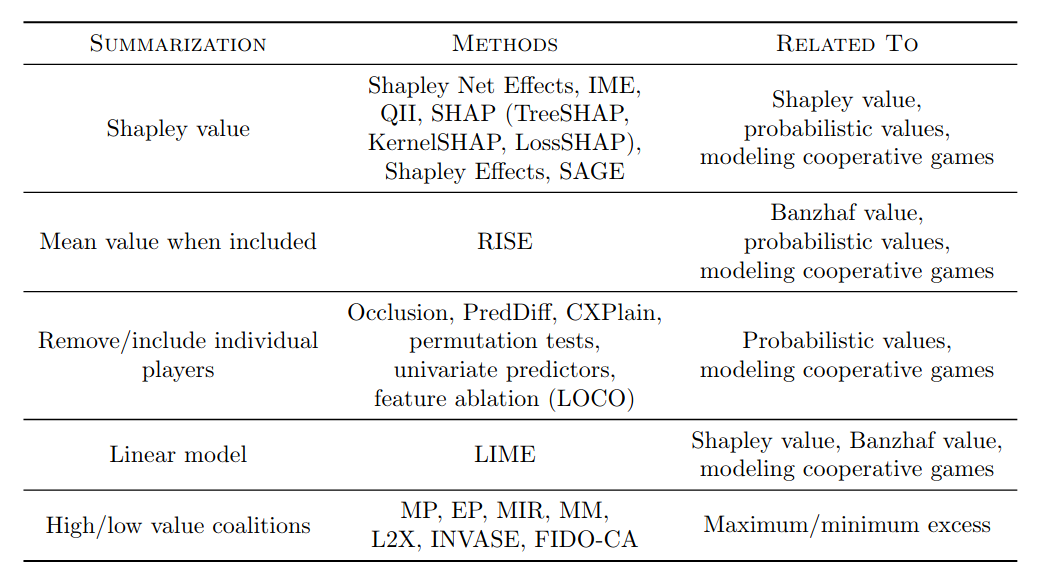 Illustration from Explaining by Removing: A Unified Framework for Model Explanation
8. Information-Theoretic Explanations
ML model $f(x) \approx p(Y \vert X = x)$ for classification, $f(x) \approx \mathbb{E}[Y \vert X = x]$ for regression (using conventional loss functions such as cross-entropy and MSE respectively).
Let’s consider $q(Y \vert X = x) \equiv f(x)$, $q(Y \vert X_S = x_S) \equiv F(x, S)$. A subset function $F$ implies a set of conditional distributions .
Here, authors show that probability axioms (countable additivity) and the Bayes rule are constraining the set of subset functions. Some will not yield a valid set of conditional distributions:
Constraining the feature removal approach to be probabilistically valid ensures that the model extension $F$ is faithful both to the original model $f$ and to an underlying data distribution.
A subset function $F \in \mathfrak{F}$ is deemed consistent with a data distribution $q(X)$ if it does not violate the countable additivity and the Bayes rule.
The authors shows that there is a unique extension $F \in \mathfrak{F}$ of a model $f \in \mathcal{F}$ that is consistent with a given data distribution $q(X)$ (cf. Propositions 6 and 7 in the paper).
This unique extension is given by
,
where $q(X_{\overline{S}} \vert X_S = x_S)$ is the conditional distribution induced by $q(X)$.
That is, if the true data distribution is $p(X)$, a consistent approach with $p$ would be to marginalize the variables. However, estimation of the conditional probability for any subset of variables is hard, and in practice one has to use approximations or assumptions such as:
- feature independence, in that case $p(X_{\overline{S}} \vert X_S = x_S) = p(X_{\overline{S}}) = \prod_{i \in \overline{S}} p(X_i)$
- model linearity (+ feature independence) corresponds to replacing removed features by their mean
- conditional generative model (e.g. a conditional GAN) which approximates the true conditional distribution
- …
This discussion shows that although few methods suggest removing features with the conditional distribution, numerous methods approximate this approach.
Training separate models should provide the best approximation because each model is given a relativelysimple task, but this is also the least scalable approach for high-dimensional datasets.
We conclude that, under certain assumptions (feature independence, model optimality), several removal strategies are consistent with the data distribution $p(X)$.
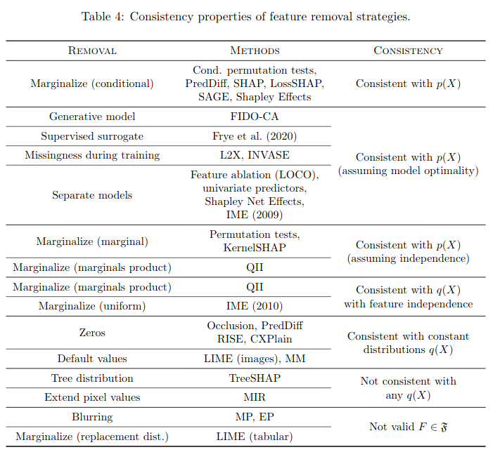 Illustration from Explaining by Removing: A Unified Framework for Model Explanation
Conventional wisdom suggests that explanation methods quantify the information contained in each feature. However, we find that precise information-theoretic connections can be identified only when removed features are marginalized out with their conditional distribution.
Given all the assumptions (consistency, i.e. features are marginalized out using the conditional distribution; optimality), the set function (extension of the model) has a probabilistic meaning, and can be tied to information-theoretic quantities such as mutual information, Kullback-Leibler divergence of the conditional probability distribution with the partial conditional probability distribution.
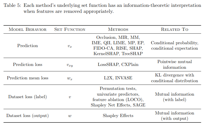 Illustration from Explaining by Removing: A Unified Framework for Model Explanation
we can view these information-theoretic quantities as the values that each set function approximates.
No single set function provides the “right” approach to model explanation; rather, these information-theoretic quantities span a range of perspectives that could be useful for understanding a complex ML model.
using ML as a tool to discover real-world relationships.
9. A Cognitive Perspective on Removal-Based Explanations
In summary, Norm theory provides a cognitive analogue for removing features by averaging over a distribution of alternative values, and the downhill rule suggests that the plausibility of alternative values should be taken into account. These theories provide cognitive justification for certain approaches to removing features, but our review of relevant psychology research is far from comprehensive. However, interestingly, our findings lend support to the same approach that yields connections with information theory (Section 8), which is marginalizing out features according to their conditional distribution.
Put simply, an explanation that paints an incomplete picture of a model may prove to be more useful if the user can understand it properly.
10. Experiments
Can check code to get a more practical understanding:
GitHub: https://github.com/iancovert/removal-explanations
Our experiments aim to accomplish three goals:
- Implement and compare many new explanation methods by partially filling out the space of removal-based explanations (recall Figure 2).
- Demonstrate the advantages of removing features by marginalizing them out using their conditional distribution.
- Validate the existence of relationships between certain explanation methods, as predicted by our previous analysis. Explanations may be similar if they use (i) summary techniques that are probabilistic values of the same cooperative game (Section 7), or (ii) feature removal strategies that are approximately equivalent (Section 8).
To cover a wide range of possible methods, we consider many combinations of removal strategies (Section 4), model behaviors (Section 5) and summary techniques (Section 6).
we implemented 80 total methods (68 of which are new)
According to Figure 9, the surrogate and Shapley value combination performs best overall; this method roughly corresponds to SAGE (Covert et al., 2020), although it uses the surrogate as an approximation of the conditional distribution.
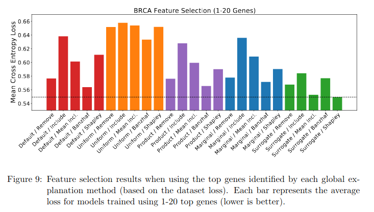 Illustration from Explaining by Removing: A Unified Framework for Model Explanation
Including individual features performs poorly, possibly because it neglects feature interactions; and removing features with uniform distributions consistently yields poor results.
However, beyond confirming known relationships, we point out that these explanations can also be used to generate new scientific hypotheses.
11. Discussion
Removal-based explanations […] specified by three precise mathematical choices:
- How the method removes features
- What model behavior the method analyzes
- How the method summarizes each feature’s influence
[…] we found that multiple model behaviors can be understood as information-theoretic quantities. These connections require that removed features are marginalized out using their conditional distribution
[…] users will not always want information-theoretic explanations. These explanations have the potentially undesirable property that features may be deemed important even if they are not used by the model in a functional sense
For practitioners:
The unique advantages of different methods are difficult to understand when each approach is viewed as a monolithic algorithm, but disentangling their choices makes it simpler to reason about their strengths and weaknesses and potentially develop hybrid methods (as demonstrated in Section 10).
For researchers:
future work will be better equipped to (i) specify the dimensions along which new methods differ from existing ones, (ii) distinguish the substance of new approaches from their approximations (to avoid presenting methods as monolithic algorithms), (iii) fix shortcomings in existing explanation methods using solutions along different dimensions of the framework, and (iv) rigorously justify new approaches in light of their connections with cooperative game theory, information theory and psychology.
Cite:
Covert, Ian, Scott Lundberg, and Su-In Lee. “Feature Removal Is a Unifying Principle for Model Explanation Methods.” arXiv preprint arXiv:2011.03623 (2020).
Books to read to get up to speed with the theory: