Hierarchical PCA x Hierarchical clustering on crypto perpetual futures
Hierarchical PCA x Hierarchical clustering on crypto perpetual futures
PCA is a useful tool for quant trading (stat arb) but in its naive implementation suffers from several forms of instabilities which yield to unnecessary turnover (trading cost…) and spurious trades.
In order to regularize the model, several techniques are available:
- Sparse PCA
- Robust PCA
- Kernel PCA
- Probabilistic PCA
- Bayesian PCA
- …
In this blog, we will discuss one in particular: The Hierarchical PCA (HPCA).
HPCA was introduced by the late Marco Avellaneda (February 16, 1955 - June 11, 2022) in Hierarchical PCA and Applications to Portfolio Management as a way to incorporate some prior knowledge (e.g. sectors) into PCA.
I already blogged about it in 2020 in this post where I replicated numerical experiments of the paper, and illustrated the impact of HPCA on the main eigenvectors obtained from stocks returns.
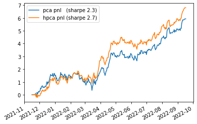
In this blog, I will apply HPCA to cryptos returns (perpetuals), and illustrate the impact it has on a downstream task (e.g. my trading book).
import numpy as np
import pandas as pd
from tqdm import tqdm
from sklearn.linear_model import LinearRegression
from scipy.cluster import hierarchy
import fastcluster
import matplotlib.pyplot as plt

def get_returns():
    """Compute daily returns from prices."""
    prices = pd.read_parquet('market_data/futures_prices.parquet')
    rect_prices = (prices
                   .pivot(index='close_time',
                          columns='symbol',
                          values='close')
                   .astype(float))

    return rect_prices.pct_change()
We will do an in-sample study on the 500 most recent days.
returns = get_returns()

xxx = returns.describe().T
coins = xxx[xxx['count'] > 500].index
returns = returns[coins].iloc[-500:]
returns.shape
(500, 101)
original_returns = returns.copy()
mean_returns = original_returns.mean()
vol_returns = original_returns.std()
We standardize the returns. PCA on standardized returns corresponds to working with the correlation matrix.
returns = returns.subtract(returns.mean(axis=0), axis=1)
returns = returns / returns.std()
Some helper function that sorts the correlation matrix:
def compute_sorted_correlations(returns, corr_estimator='pearson'):
    corr = returns.corr(method=corr_estimator)
    dist = 1 - corr.values
    tri_a, tri_b = np.triu_indices(len(dist), k=1)
    linkage = fastcluster.linkage(dist[tri_a, tri_b], method='ward')
    permutation = hierarchy.leaves_list(
        hierarchy.optimal_leaf_ordering(linkage, dist[tri_a, tri_b]))
    sorted_coins = returns.columns[permutation]
    sorted_corrs = corr.values[permutation, :][:, permutation]

    return pd.DataFrame(sorted_corrs, index=sorted_coins, columns=sorted_coins)
sorted_correlations = compute_sorted_correlations(returns)
returns = returns[sorted_correlations.columns.tolist()]
plt.pcolormesh(sorted_correlations)
plt.colorbar()
plt.title('Sorted correlation matrix')
plt.show()
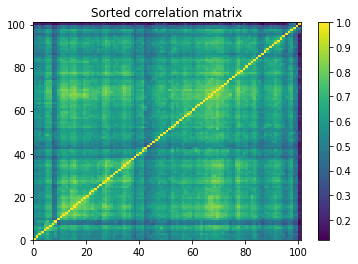
We can notice that there are no obvious correlation clusters.
Applying Hierarchical PCA on this dataset may not be such a good idea: HPCA is supposed to help stabilise PCA when there are obvious groupings of assets. If there are none, then it may impose a spurious structure…
Let’s continue nonetheless this exercise.
corr = returns.corr().values
tri_a, tri_b = np.triu_indices(len(corr), k=1)
flat_corr = corr[tri_a, tri_b]
plt.hist(flat_corr, bins=100)
plt.axvline(flat_corr.mean(), color='k')
plt.show()
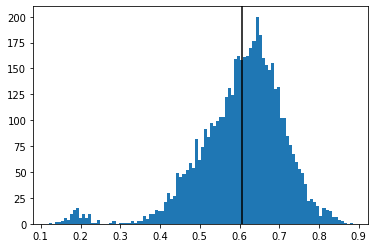
One can observe that these 101 cryptos are very correlated on average, at the exception of 2 or 3 tokens.
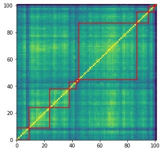
Let’s overlay (the somewhat spurious) 10 clusters on top of the correlation matrix, and save their members for later:
nb_clusters = 10
dist = 1 - sorted_correlations.values
dim = len(dist)
tri_a, tri_b = np.triu_indices(dim, k=1)
linkage = fastcluster.linkage(dist[tri_a, tri_b], method='ward')
clustering_inds = hierarchy.fcluster(linkage, nb_clusters,
criterion='maxclust')
clusters = {i: [] for i in range(min(clustering_inds),
max(clustering_inds) + 1)}
for i, v in enumerate(clustering_inds):
clusters[v].append(i)
permutation = sorted([(min(elems), c) for c, elems in clusters.items()],
key=lambda x: x[0], reverse=False)
sorted_clusters = {}
for cluster in clusters:
sorted_clusters[cluster] = clusters[permutation[cluster - 1][1]]
plt.figure(figsize=(5, 5))
plt.pcolormesh(sorted_correlations)
for cluster_id, cluster in sorted_clusters.items():
xmin, xmax = min(cluster), max(cluster)
ymin, ymax = min(cluster), max(cluster)
plt.axvline(x=xmin,
ymin=ymin / dim, ymax=(ymax + 1) / dim,
color='r')
plt.axvline(x=xmax + 1,
ymin=ymin / dim, ymax=(ymax + 1) / dim,
color='r')
plt.axhline(y=ymin,
xmin=xmin / dim, xmax=(xmax + 1) / dim,
color='r')
plt.axhline(y=ymax + 1,
xmin=xmin / dim, xmax=(xmax + 1) / dim,
color='r')
plt.show()
coin_to_cluster = {}
for cluster in sorted_clusters:
print('Cluster', cluster)
cluster_members = sorted_correlations.columns[sorted_clusters[cluster]].tolist()
for coin in cluster_members:
coin_to_cluster[coin] = cluster
print(f'size: {len(cluster_members)}')
print(cluster_members)
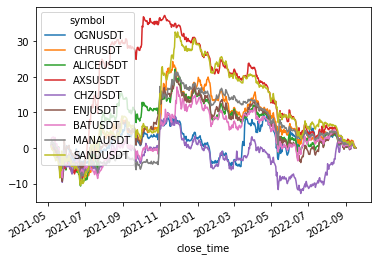
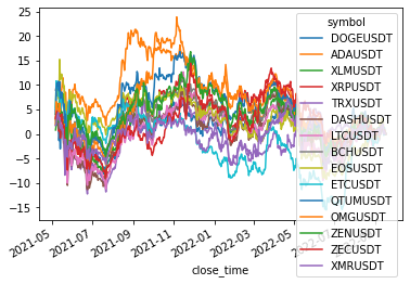
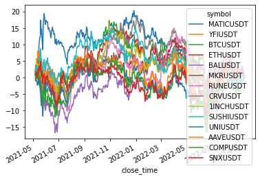
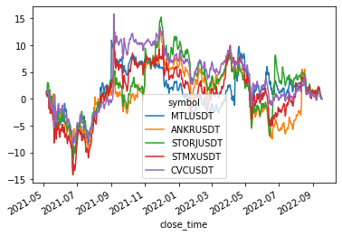
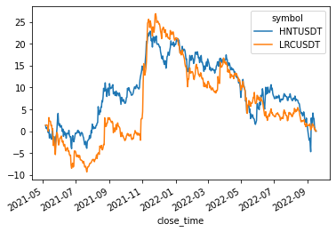
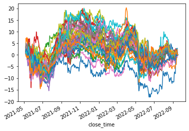
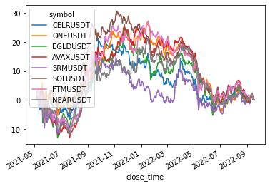
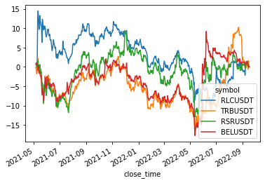
returns[cluster_members].cumsum().plot(legend=(len(cluster_members) < 20))
plt.show()
# everything is sorted, no need to preserve old permutation
returns.columns = sorted_correlations.columns
sorted_correlations.columns = sorted_correlations.columns
sorted_correlations.index = sorted_correlations.columns
Cluster 1
size: 9
['OGNUSDT', 'CHRUSDT', 'ALICEUSDT', 'AXSUSDT', 'CHZUSDT', 'ENJUSDT', 'BATUSDT', 'MANAUSDT', 'SANDUSDT']
Cluster 2
size: 15
['DOGEUSDT', 'ADAUSDT', 'XLMUSDT', 'XRPUSDT', 'TRXUSDT', 'DASHUSDT', 'LTCUSDT', 'BCHUSDT', 'EOSUSDT', 'ETCUSDT', 'QTUMUSDT', 'OMGUSDT', 'ZENUSDT', 'ZECUSDT', 'XMRUSDT']
Cluster 3
size: 14
['MATICUSDT', 'YFIUSDT', 'BTCUSDT', 'ETHUSDT', 'BALUSDT', 'MKRUSDT', 'RUNEUSDT', 'CRVUSDT', '1INCHUSDT', 'SUSHIUSDT', 'UNIUSDT', 'AAVEUSDT', 'COMPUSDT', 'SNXUSDT']
Cluster 4
size: 5
['MTLUSDT', 'ANKRUSDT', 'STORJUSDT', 'STMXUSDT', 'CVCUSDT']
Cluster 5
size: 2
['HNTUSDT', 'LRCUSDT']
Cluster 6
size: 42
['CTKUSDT', 'LITUSDT', 'TOMOUSDT', 'SKLUSDT', 'LINAUSDT', 'NKNUSDT', 'ZILUSDT', 'IOSTUSDT', 'ALGOUSDT', 'HBARUSDT', 'RVNUSDT', 'REEFUSDT', 'DGBUSDT', 'HOTUSDT', 'DENTUSDT', 'FILUSDT', 'IOTAUSDT', 'ICXUSDT', 'THETAUSDT', 'GRTUSDT', 'SXPUSDT', 'ONTUSDT', 'NEOUSDT', 'BNBUSDT', 'VETUSDT', 'LINKUSDT', 'BANDUSDT', 'XEMUSDT', 'ZRXUSDT', 'FLMUSDT', 'BLZUSDT', 'ALPHAUSDT', 'DOTUSDT', 'KSMUSDT', 'OCEANUSDT', 'RENUSDT', 'ATOMUSDT', 'XTZUSDT', 'KAVAUSDT', 'COTIUSDT', 'KNCUSDT', 'WAVESUSDT']
Cluster 7
size: 8
['CELRUSDT', 'ONEUSDT', 'EGLDUSDT', 'AVAXUSDT', 'SRMUSDT', 'SOLUSDT', 'FTMUSDT', 'NEARUSDT']
Cluster 8
size: 4
['RLCUSDT', 'TRBUSDT', 'RSRUSDT', 'BELUSDT']
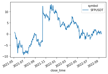
Cluster 9
size: 1
['SFPUSDT']
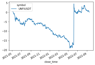
Cluster 10
size: 1
['UNFIUSDT']
Hierarchical PCA
HPCA consists in pre-processing the correlation matrix before applying a standard PCA on top of it.
HPCA computes the first eigenvector $v_1^{j}$ of each cluster $j$, then overrides the inter-cluster correlations by the (adjusted) correlation between their respective factor $F_1^j = \frac{1}{\sqrt{\lambda_1^j}} X_{j} v_1^j$, leaving the intra-cluster correlations untouched.
The code below computes $F_1^j$ for each cluster $j$, and stores it for further processing:
eigen_clusters = {}
for cluster in clusters:
    cluster_members = sorted_correlations.columns[
        sorted_clusters[cluster]].tolist()
    corr_cluster = sorted_correlations.loc[
        cluster_members, cluster_members]

    cluster_returns = returns[cluster_members]

    eigenvals, eigenvecs = np.linalg.eig(corr_cluster.values)

    idx = eigenvals.argsort()[::-1]
    eigenvals = eigenvals[idx]
    eigenvecs = eigenvecs[:, idx]

    val1 = eigenvals[0]
    vec1 = eigenvecs[:, 0]
    F1 = (1 / np.sqrt(val1)) * np.multiply(
        vec1, cluster_returns.values).sum(axis=1)

    eigen_clusters[cluster] = {
        'tickers': cluster_members,
        'val1': val1,
        'vec1': vec1,
        'F1': F1,}
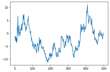
Cumulative returns of $F_1^3$ (as a mere illustration):
plt.plot(eigen_clusters[3]['F1'].cumsum());
Coins in a given cluster $j$ may have different sensitivity to $F_1^j$.
We can obtain the sensitivity $\beta_k^j$ of coin $k$ member of cluster $j$ to its associated factor $F_1^j$ with a simple linear regression:
betas = {}
for coin in returns.columns:

    coin_returns = returns[coin]
    cluster_F1 = eigen_clusters[coin_to_cluster[coin]]['F1']

    reg = LinearRegression(fit_intercept=False).fit(
        cluster_F1.reshape(-1, 1), coin_returns)

    beta = reg.coef_[0]

    betas[coin] = beta
We have now all the pieces to transform the correlation matrix according to the HPCA algorithm:
HPCA_corr = sorted_correlations.copy()
for coin_1 in HPCA_corr.columns:
    beta_1 = betas[coin_1]
    F1_1 = eigen_clusters[coin_to_cluster[coin_1]]['F1']
    for coin_2 in HPCA_corr.columns:
        beta_2 = betas[coin_2]
        F1_2 = eigen_clusters[coin_to_cluster[coin_2]]['F1']
        if coin_to_cluster[coin_1] != coin_to_cluster[coin_2]:
            rho_sector = np.corrcoef(F1_1, F1_2)[0, 1]
            mod_rho = beta_1 * beta_2 * rho_sector
            HPCA_corr.at[coin_1, coin_2] = mod_rho
            HPCA_corr.at[coin_1, coin_2] = mod_rho
plt.figure(figsize=(16, 6))
plt.subplot(1, 2, 1)
plt.pcolormesh(sorted_correlations)
plt.colorbar()
plt.title('Correlation matrix with clustering order')

plt.subplot(1, 2, 2)
plt.pcolormesh(HPCA_corr)
plt.colorbar()
plt.title('HPCA correlation matrix with clustering order')
plt.show()
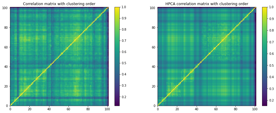
The inter-correlations are cleaner than the intra-correlations (left untouched).
It might be worthwhile to try variations of this HPCA algorithm, filtering intra-correlations as well.
Let’s now compare PCA and HPCA:
eigenvals, eigenvecs = np.linalg.eig(sorted_correlations.values)

idx = eigenvals.argsort()[::-1]
pca_eigenvals = eigenvals[idx]
pca_eigenvecs = eigenvecs[:, idx]

eigenvals, eigenvecs = np.linalg.eig(HPCA_corr.values)

idx = eigenvals.argsort()[::-1]
hpca_eigenvals = eigenvals[idx]
hpca_eigenvecs = eigenvecs[:, idx]
plt.figure(figsize=(10, 5))
plt.plot(np.cumsum(pca_eigenvals) / pca_eigenvals.sum(), label='PCA')
plt.plot(np.cumsum(hpca_eigenvals) / hpca_eigenvals.sum(), label='HPCA')
plt.axhline(1, color='k')
plt.xlabel('rank k of eigenvalue')
plt.ylabel('variance explained')
plt.title('Variance explained = ' +
          'sum of the k largest eigenvalues / sum of all eigenvalues')
plt.legend()
plt.show()
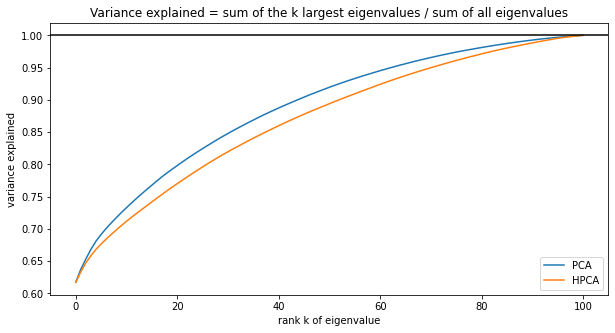
Unsurprisingly, one needs more HPCA components to explain the same amount of variance compared to PCA (due to the filtering). PCA may just overfit (as optimal in-sample with respect to variance maximization, by definition).
Let’s look into the first 10 eigenvectors:
for i in range(10):
    fig, ax = plt.subplots(figsize=(15, 5),
                           tight_layout=True)
    corr_pcs = np.corrcoef(pca_eigenvecs[:, i],
                           hpca_eigenvecs[:, i])[0, 1]
    if corr_pcs < 0:
        hpca_eigenvecs[:, i] = -hpca_eigenvecs[:, i]

    plt.plot(pca_eigenvecs[:, i], label='PCA')
    plt.plot(hpca_eigenvecs[:, i], label='HPCA')
    plt.title('Eigenvector {} -- '.format(i + 1) +
              'Correlation between PC{} and HPC{} = {}'.format(
        i + 1, i + 1, round(abs(corr_pcs), 2)), fontsize=14)
    plt.legend()
    plt.show()
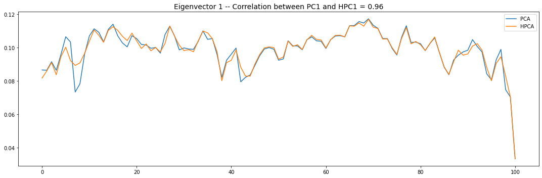
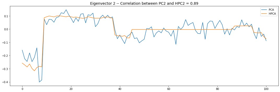
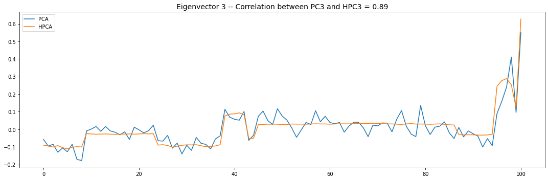
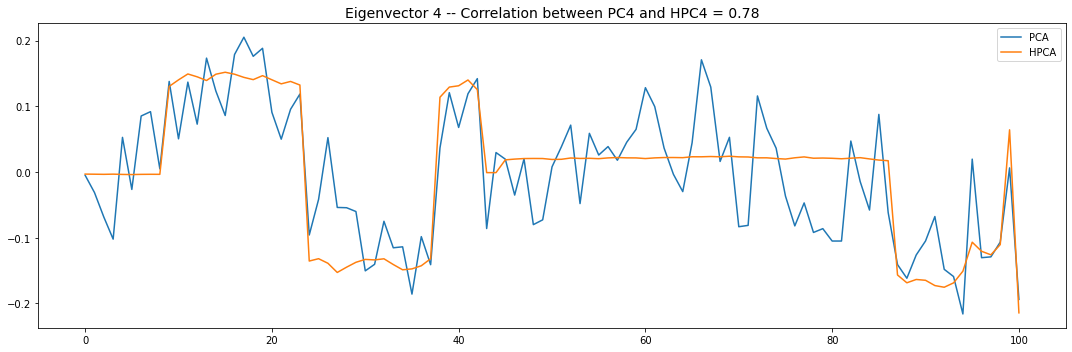
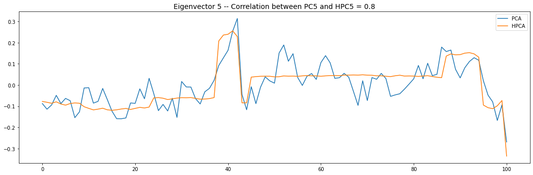
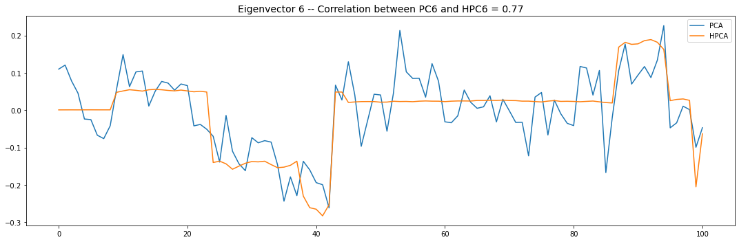
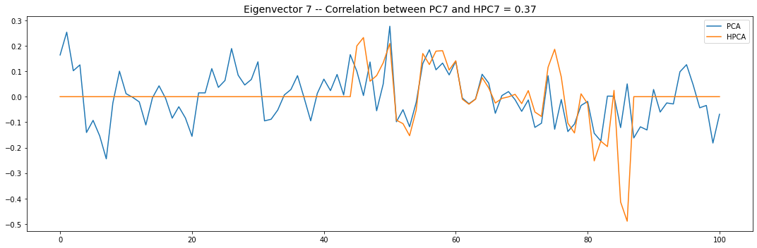
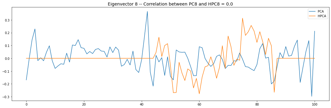
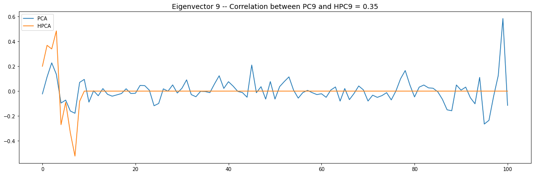
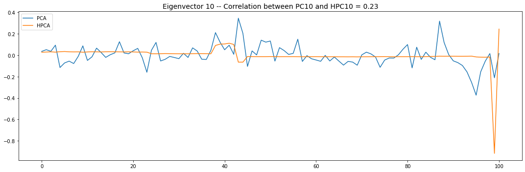
PCA and HPCA agree to a large extent.
Eigenvectors obtained from HPCA exhibit more regularity which is enforced by construction when using the clustering to pre-process the correlation matrix.
Is it a good thing in practice?
I believe the answer to this question is very much application-specific.
If anything, when plugging Hierarchical PCA (instead of PCA) in my crypto trading book, I obtained a surprising boost in performance that I did not expect (since there is no blatant clustering structure between the liquid perpetuals - at the exception of GameFi)…