Quick correlation study between BTC/USD and ETH/USD
import numpy as np
import scipy
import pandas as pd
import matplotlib.pyplot as plt
%matplotlib inline
import seaborn as sns
import json
from datetime import timedelta
You can find and save yourself the data thanks to the cryptocompare API. Here, I select the pair BTC/USD (first link) and a daily aggregate (&aggregate=1&e=CCCAGG). I do the same for the ETH/USD pair.
- https://min-api.cryptocompare.com/data/histoday?fsym=BTC&tsym=USD&limit=600000000000&aggregate=1&e=CCCAGG
- https://min-api.cryptocompare.com/data/histoday?fsym=ETH&tsym=USD&limit=600000000000&aggregate=1&e=CCCAGG
data_BTC = []
with open('BTCUSD.json') as f:
    for line in f:
        data_BTC.append(json.loads(line))

data_ETH = []
with open('ETHUSD.json') as f:
    for line in f:
        data_ETH.append(json.loads(line))

histo_BTC = pd.DataFrame(data_BTC)
histo_ETH = pd.DataFrame(data_ETH)

histo_ETH['time'] = pd.to_datetime(histo_ETH['time'],unit='s')
histo_BTC['time'] = pd.to_datetime(histo_BTC['time'],unit='s')

histo_ETH.index = histo_ETH['time']
histo_BTC.index = histo_BTC['time']
histo_ETH.tail()
| close | high | low | open | time | volumefrom | volumeto | |
|---|---|---|---|---|---|---|---|
| time | |||||||
| 2017-08-18 | 292.62 | 306.52 | 287.17 | 300.30 | 2017-08-18 | 523133.90 | 1.553331e+08 |
| 2017-08-19 | 293.02 | 298.79 | 283.65 | 292.62 | 2017-08-19 | 458296.55 | 1.333319e+08 |
| 2017-08-20 | 298.20 | 298.78 | 288.48 | 293.02 | 2017-08-20 | 293661.68 | 8.621471e+07 |
| 2017-08-21 | 321.85 | 345.44 | 294.93 | 298.20 | 2017-08-21 | 1147950.71 | 3.713201e+08 |
| 2017-08-22 | 315.09 | 329.39 | 293.09 | 321.85 | 2017-08-22 | 728103.98 | 2.256794e+08 |
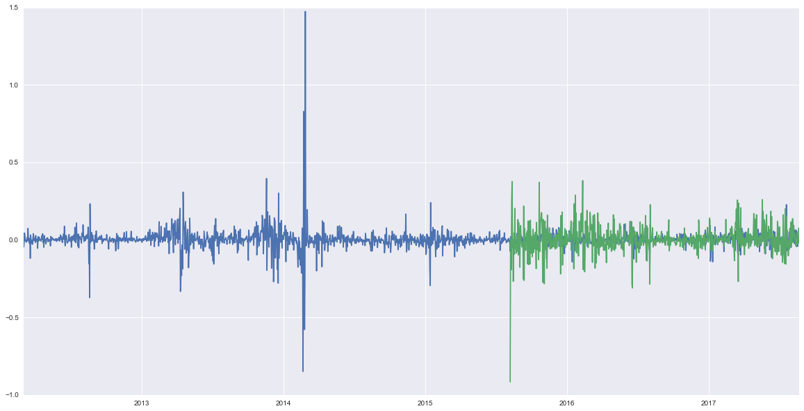
We compute the log returns from the prices:
returns_BTC = pd.DataFrame(np.diff(np.log(histo_BTC['close'].get_values()),axis=0))
returns_BTC.index = histo_BTC.index[1:]
returns_BTC.columns = ['returns']

returns_ETH = pd.DataFrame(np.diff(np.log(histo_ETH['close'].get_values()),axis=0))
returns_ETH.index = histo_ETH.index[1:]
returns_ETH.columns = ['returns']
plt.figure(figsize=(20,10))
plt.plot(returns_BTC)
plt.plot(returns_ETH)
plt.show()
Then, we are going to compute the correlation on a rolling window of 60 consecutive days:
start_date = returns_BTC.index[0]
window_length = timedelta(days=60)
step_length = timedelta(days=1)

correls = []
start_window = start_date
while start_window + window_length <= histo_BTC.index[-1]:
    end_window = start_window + window_length

    window_returns_BTC = returns_BTC.loc[start_window:end_window]
    window_returns_ETH = returns_ETH.loc[start_window:end_window]

    correl = np.corrcoef(window_returns_BTC.values.flatten(),
                         window_returns_ETH.values.flatten(),
                         "spearman")[0,1]
    correls.append(correl)
    start_window += step_length

correl_df = pd.DataFrame(correls,index=returns_BTC.loc[start_date+window_length:].index,columns=['corr'])
plt.figure(figsize=(25,10))
ax = plt.gca()
ax2 = ax.twinx()
plt.axis('normal')
ax.plot(histo_ETH['close'])
ax.plot(histo_BTC['close'])
ax2.plot(correl_df,color='red')
ax.set_ylabel("crypto rates",fontsize=14,color='blue')
ax2.set_ylabel("correlation",fontsize=14,color='blue')
ax.grid(True)
plt.title("ETH/USD and BTC/USD rates and their correlation", fontsize=20,color='black')
ax.set_xlabel('time', fontsize=14, color='b')
ax.legend(['ETH/USD','BTC/USD'],loc='best')
ax2.legend(['correl(BTC,ETH)'],loc='upper right')
plt.show()
Here is the result:
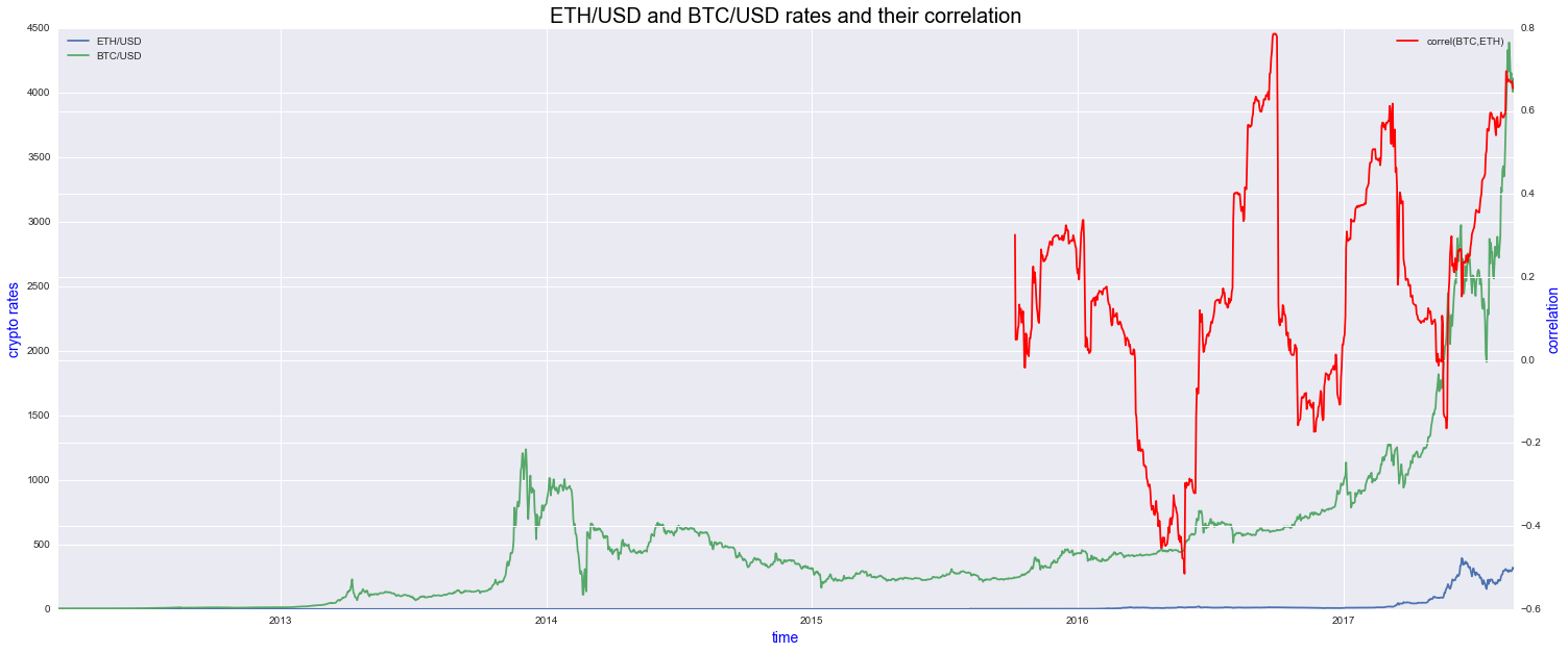
Correlation between the two pairs is nearly at an all time high!