How to detect false strategies? The Deflated Sharpe Ratio
Deflated Sharpe Ratio
In this blog post, we implement the deflated sharpe ratio as described in the following papers:
The Sharpe Ratio (SR) is one of the most widely used statistic for measuring the performance of a strategy / manager / fund. In its most simplistic definition, it is defined as the historical excess returns $\mu$ normalized by the realized risk (volatility of the returns) $\sigma$, thus $SR = \frac{\mu}{\sigma}$.
When datamining strategies, the more backtests computed the more likely a spurious strategy having high Sharpe ratio can be found.
Expected Maximum Sharpe Ratio
Given a strategy class, authors of the previously cited papers assume that the Sharpe ratio estimates of the $N$ trials ${\hat{SR}_n}, n=1, \ldots, N$ follow a Normal distribution with mean $\mathbf{E}[{\hat{SR}_n}]$ and variance $\mathbf{V}[{\hat{SR}_n}]$. Under these assumptions, they show that the expected maximum of ${\hat{SR}_n}$ after $N \gg 1$ independent trials can be approximated by:
where $\gamma$ ($\approx 0.5772$) is the Euler-Mascheroni constant, $Z$ is the cumulative function of the standard Normal distribution, and $e$ is Euler’s number.
Let’s play a bit with this approximation to see
-
how accurate the analytical formula is with respect to empirical estimates of $\mathbf{E}[\max {\hat{SR}_n}]$;
-
how big a Sharpe ratio estimate can be for a variance of 1 and a true Sharpe ratio of 0.
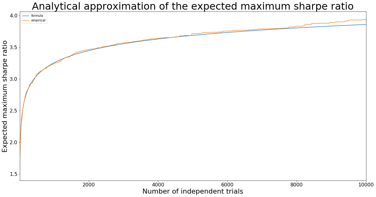
Accuracy of the Expected Maximum Sharpe Ratio formula
import pandas as pd
import numpy as np
from scipy.stats import norm
import matplotlib.pyplot as plt
%matplotlib inline

# universal constants
gamma = 0.5772156649015328606
e = np.exp(1)

# analytical formula for expected maximum sharpe ratio
def approximate_expected_maximum_sharpe(mean_sharpe, var_sharpe, nb_trials):
    return mean_sharpe + np.sqrt(var_sharpe) * (
        (1 - gamma) * norm.ppf(1 - 1 / nb_trials) + gamma * norm.ppf(1 - 1 / (nb_trials * e)))
nb_samples = 10**2
max_nb_trials = 10**4 + 1
step_nb_trials = 10

mean_sharpe = 0
var_sharpe = 1 / 252
std_sharpe = np.sqrt(var_sharpe)


formula_sharpes = pd.Series(
    [approximate_expected_maximum_sharpe(
        mean_sharpe, var_sharpe, nb_trials) * np.sqrt(252)
     for nb_trials in range(10, max_nb_trials, step_nb_trials)],
    index=range(10, max_nb_trials, step_nb_trials),
    name='formula')


sharpe_estimates = np.random.normal(mean_sharpe, std_sharpe, (nb_samples, max_nb_trials))
empirical_sharpes = pd.Series(
    [np.mean([max(sharpe_estimates[sample, :nb_trials]) * np.sqrt(252)
             for sample in range(nb_samples)])
     for nb_trials in range(10, max_nb_trials, step_nb_trials)],
    index=range(10, max_nb_trials, step_nb_trials),
    name='empirical')
expected_max_sharpes = pd.concat([formula_sharpes, empirical_sharpes], axis=1)

ax = expected_max_sharpes.plot(title='Analytical approximation of the expected maximum sharpe ratio',
                               figsize=(20,10), fontsize=16)
ax.set_xlabel('Number of independent trials', fontsize=22)
ax.set_ylabel('Expected maximum sharpe ratio', fontsize=22)
ax.title.set_size(32)
Examples of Expected Maximum Sharpe Ratios for fluke strategies
mean_sharpe = 0
var_sharpe = 1 / 252
std_sharpe = np.sqrt(var_sharpe)


# number of independent trials
nb_trials = 100
nb_samples = 10**4


formula_expected_max_sharpe = approximate_expected_maximum_sharpe(mean_sharpe,
                                                                  var_sharpe,
                                                                  nb_trials)

print("Formula Expected Maximum Sharpe Ratio (annualized): ",
      round(formula_expected_max_sharpe * np.sqrt(252), 2))


sharpe_estimates = np.random.normal(0, std_sharpe, (nb_samples, nb_trials))

print("Empirical Expected Maximum Sharpe Ratio (annualized): ",
      round(np.mean([max(sharpe_estimates[sample,]) * np.sqrt(252)
                     for sample in range(nb_samples)]), 2))
Formula Expected Maximum Sharpe Ratio (annualized):  2.53
Empirical Expected Maximum Sharpe Ratio (annualized):  2.5
It means that after only 100 trials, we can find a strategy having a Sharpe ratio of 2.5 in backtesting (whereas the true value is 0, i.e. the strategy should not earn any money). Formula and empirical values for the expected maximum Sharpe ratio are pretty close.
Let’s see how the expected maximum Sharpe ratio varies with an increasing standard deviation of the Sharpe ratio Normal distribution.
mean_sharpe = 0
var_sharpes = [annual_var / 252 for annual_var in [1, 4, 10]]
std_sharpes = [np.sqrt(var_sharpe) for var_sharpe in var_sharpes]

max_nb_trials = 10**3 + 1
step_nb_trials = 5

expected_max_sharpes = pd.DataFrame(
    [[approximate_expected_maximum_sharpe(
        mean_sharpe, var_sharpe, nb_trials) * np.sqrt(252)
      for var_sharpe in var_sharpes]
     for nb_trials in range(10, max_nb_trials, step_nb_trials)],
    index=range(10, max_nb_trials, step_nb_trials),
    columns=[round(std_sharpe, 2) for std_sharpe in std_sharpes])
ax = expected_max_sharpes.plot(title='Expected maximum sharpe ratio by standard deviation',
                               figsize=(20, 10), fontsize=16)
ax.set_xlabel('Number of independent trials', fontsize=22)
ax.set_ylabel('Expected maximum sharpe ratio', fontsize=22)
ax.title.set_size(32)
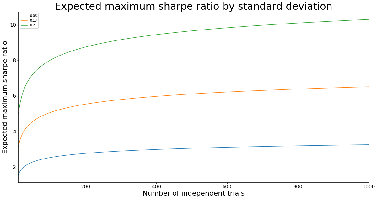
As expected, with increasing variance of the Sharpe ratio distribution, it is more likely to obtain higher Sharpe ratios for a given number of independent trials.
Deflated Sharpe Ratio
The Deflated Sharpe Ratio (DSR) is defined as:
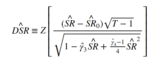
where $\hat{SR}_0 = \sqrt{\mathbf{V}[{\hat{SR}_n}]} \left( (1 - \gamma) Z^{-1} \left[ 1 - \frac{1}{N} \right] + \gamma Z^{-1} \left[ 1 - \frac{1}{N}e^{-1} \right] \right)$, $\mathbf{V}[{\hat{SR}_n}]$ is the variance across the trials, and $N$ the number of independent trials.
$\hat{SR}_0$ is the Expected Maximum Sharpe Ratio (analytical formula) for a Sharpe ratio Normal distribution centered on $\mathbf{E}[{\hat{SR}_n}] = 0$, used here as a null hypothesis.
The formula above gives the probability that the true Sharpe ratio (SR) is above $\hat{SR}_0$, i.e. that the true Sharpe ratio is positive.
The Deflated Sharpe Ratio depends on
-
the estimated Sharpe ratio $\hat{SR}$,
-
the sample size $T$, e.g. on how many trading days $T$ the strategy has been backtested,
-
the first four moments of the alpha / strategy / manager / fund returns to discount for exceptional returns.
def compute_deflated_sharpe_ratio(*,
                                  estimated_sharpe,
                                  sharpe_variance,
                                  nb_trials,
                                  backtest_horizon,
                                  skew,
                                  kurtosis):
    SR0 = approximate_expected_maximum_sharpe(0, sharpe_variance, nb_trials)

    return norm.cdf(((estimated_sharpe - SR0) * np.sqrt(backtest_horizon - 1))
                    / np.sqrt(1 - skew * estimated_sharpe + ((kurtosis - 1) / 4) * estimated_sharpe**2))
A (potentially) spurious strategy
Let’s consider a strategy that has a 2.5 annual Sharpe ratio. This strategy was chosen after 100 trials, with a Sharpe ratio variance of 0.5 when estimated on these 100 trials. To claim that the strategy has a 2.5 Sharpe ratio, it was backtested on 1250 trading days. In the backtesting, the returns of this strategy have a skewness of -3 and a kurtosis of 10.
Question: What is the probability that this strategy is totally spurious?
compute_deflated_sharpe_ratio(estimated_sharpe=2.5 / np.sqrt(252),
                              sharpe_variance=0.5 / 252,
                              nb_trials=100,
                              backtest_horizon=1250,
                              skew=-3,
                              kurtosis=10)
0.89967234849777633
There is only a 90% chance that the advertized strategy has a positive Sharpe ratio. Put another way, there is a 10% chance that the strategy does not earn money at all (despite being advertized with a pretty good Sharpe ratio of 2.5).