Network-based vs. Minimum Variance portfolios: Any deep connections?
Network-based vs. Minimum Variance portfolios: Any deep connections?
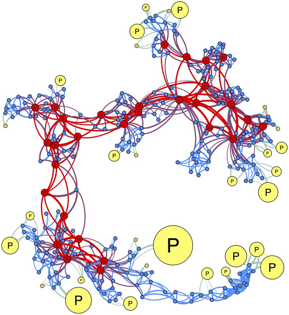
Researchers from the complex networks (applied in finance) community have noticed that the biggest weights of a Minimum Variance portfolio are associated to stocks that are located on the outskirts of a correlation network (for example, the leaves of a minimum spanning tree). In Spread of risk across financial markets: better to invest in the peripheries, authors suggest to invest in stocks that occupy peripheral, poorly connected regions in correlation filtered networks. We can see in the figure below (from the mentioned article) the connection between the outskirts of the correlation network and the Markowitz weights: The more peripheral, the bigger the weights (size of the nodes).
One can thus wonders whether there are connections between the two approaches. Maybe the two approaches are two different descriptions of an underlying similar objective function? In Portfolio selection based on graphs: Does it align with Markowitz-optimal portfolios?, Hüttner et al. study this question.
TL;DR No, the two methods are quite different. The fact that the empirical literature finds that they give similar results may come from the data itself, i.e. a stylized fact of financial correlations. The relation does not hold in general for random correlation matrices.
Relation between Minimum Variance portfolio and eigenvector centrality
There exist several definitions of centraliy in networks. We here use the one mentioned in the article (eigenvector centrality): lambda v = C v, where v is the centrality vector, lambda the highest eigenvalue of C the correlation matrix defining the weighted network.
import numpy as np
from multiprocessing import Pool
from numpy.random import beta
from numpy.random import randn
from scipy.linalg import sqrtm
from numpy.random import seed
from tqdm import tqdm
import matplotlib.pyplot as plt
%matplotlib inline

seed(42)
def compute_mv_weights(C):
    ones = np.ones(len(C))
    inv_C = np.linalg.inv(C)

    return (np.dot(inv_C, ones) /
            np.dot(ones, np.dot(inv_C, ones)))

def compute_eigenvector_centrality(C):
    eigenvals, eigenvecs = np.linalg.eig(C)
    fst_eigenvec = eigenvecs[:, np.argmax(eigenvals)]

    return fst_eigenvec / np.sum(fst_eigenvec)
To study if there is a relation between the Minimum Variance Portfolio (MVP) and eigenvector centrality in general, we will compute some statistics of the resulting MVP and estimated centralities given a correlation matrix in input, and verify if these statistics are similar.
More precisely, we will sample uniformly correlation matrices from the whole space of correlation matrices (cf. the blog post How to sample uniformly over the space of correlation matrices? The onion method); Then, following the article, we will compute the “portfolio weight of the 20% least central assets”. If the centrality measure were independent of the MVP weights, then this quantity should be 20%. If the centrality measure tends to pick the same assets as the MVP, this quantity should be more than 20%.
For convenience, and following the article, we normalize the quantity “portfolio weight of the 20% least central assets” by 0.2. Therefore, we want to verify if the ratio is significantly above 1 or not.
def sample_unif_correlmat(dimension):
    d = dimension + 1

    prev_corr = np.matrix(np.ones(1))
    for k in range(2, d):
        # sample y = r^2 from a beta distribution with alpha_1 = (k-1)/2 and alpha_2 = (d-k)/2
        y = beta((k - 1) / 2, (d - k) / 2)
        r = np.sqrt(y)

        # sample a unit vector theta uniformly from the unit ball surface B^(k-1)
        v = randn(k-1)
        theta = v / np.linalg.norm(v)

        # set w = r theta
        w = np.dot(r, theta)

        # set q = prev_corr**(1/2) w
        q = np.dot(sqrtm(prev_corr), w)

        next_corr = np.zeros((k, k))
        next_corr[:(k-1), :(k-1)] = prev_corr
        next_corr[k-1, k-1] = 1
        next_corr[k-1, :(k-1)] = q
        next_corr[:(k-1), k-1] = q

        prev_corr = next_corr

    return prev_corr
def compute_stat_1(C, p=0.2):
    MVP_weights = compute_mv_weights(C)
    centralities = compute_eigenvector_centrality(C)
    # find the k (20%) smallest values
    k = int(len(C) * p)
    idx = centralities.argsort()[:k]

    return MVP_weights[idx].sum() / p
nb_samples = 5000
list_nb_assets = [5, 10, 50, 100, 200]

ratios = {}
for nb_assets in list_nb_assets:

    correlmats = [sample_unif_correlmat(nb_assets)
                  for sample in tqdm(range(nb_samples))]

    with Pool() as pool:
        values = list(
            tqdm(pool.imap_unordered(compute_stat_1,
                                     correlmats),
                 total=nb_samples))

    ratios[nb_assets] = values
100%|██████████| 5000/5000 [00:04<00:00, 1241.84it/s]
100%|██████████| 5000/5000 [00:00<00:00, 8926.84it/s]
100%|██████████| 5000/5000 [00:08<00:00, 568.94it/s]
100%|██████████| 5000/5000 [00:00<00:00, 10125.27it/s]
100%|██████████| 5000/5000 [05:18<00:00, 15.71it/s]
100%|██████████| 5000/5000 [00:08<00:00, 616.97it/s]
100%|██████████| 5000/5000 [42:39<00:00,  1.95it/s]
100%|██████████| 5000/5000 [01:10<00:00, 70.76it/s]
100%|██████████| 5000/5000 [3:51:05<00:00,  2.77s/it]
100%|██████████| 5000/5000 [04:34<00:00, 18.24it/s]
for d in list_nb_assets:
    density, edges, hist = plt.hist(ratios[d],
                                    bins=10000,
                                    density=True,
                                    stacked=True)
    proba = sum([v for (v, b) in zip(density, edges)
                 if b <= 1]) * (edges[1] - edges[0])

    plt.clf()
    plt.title("d = " + str(d) + ", mean = "
              + str(round(np.mean(ratios[d]), 2))
              + ", proba(stat < 1) = " + str(round(np.mean(proba), 2)))
    plt.hist(ratios[d], bins=100, range=(-4, 4))
    plt.plot()
    plt.show()
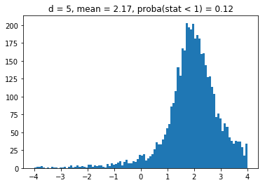
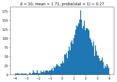
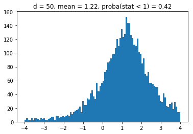
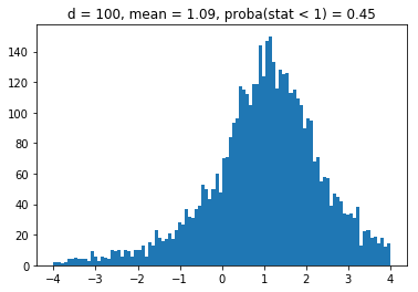
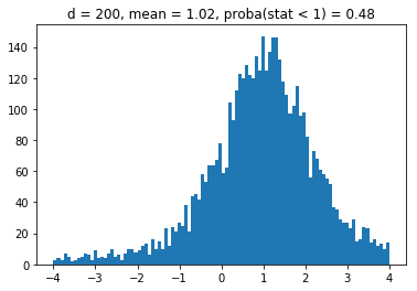
We obtain results similar to the paper: It seems that the higher the dimension (the number of assets), the less likely it is that the least central assets will be overrepresented in the MVP as (with growing dimension) the distributions obtained seem more and more symmetric and centered on 1.
So far, only considering eigenvector centrality, it doesn’t seem that MVP and network-based methods select the same subset of assets in general. However, we only considered one possible definition of centrality in a network, which was until now defined implicitely. In the next blog post, we will explore other definitions of centrality applied to an explicitely built correlation filtering network: the Minimum Spanning Tree.