Hierarchical Risk Parity - Implementation & Experiments (Part II)
Hierarchical Risk Parity - Implementation & Experiments (Part II)
This blog follows Hierarchical Risk Parity - Implementation & Experiments (Part I) in which we implemented the ``Hierarchical Risk Parity’’ (HRP) approach proposed by Marcos Lopez de Prado in his paper Building Diversified Portfolios that Outperform Out-of-Sample and his book Advances in Financial Machine Learning.
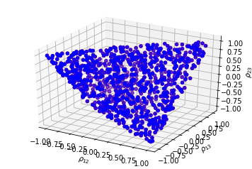
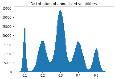
In this blog, we compare the Hierarchical Risk Parity and standard naive approaches such as Equal Weighting, Risk Parity and Minimum Variance on in- and out-samples. Synthetic returns are drawn from a centered Gaussian (taily distributions will be used in a following post, let’s keep it simple for now) parameterized by a random covariance matrix, where the variances are sampled from a multimodal distribution and the underlying correlation matrix from the uniform distribution over the space of correlation matrices using the onion method, an algorithm described in this previous blog post.
The goal of these simulations is to study the stability of the different methods between their in- and out-sample results.
TL;DR HRP is relatively stable. In these simulations, HRP may suffer from the lack of true hierarchical clusters, so working on an arbitrary order based on the clusters it finds spuriously in the noise. Therefore HRP has a relatively close behaviour, yet subpar out of sample, to the naive Risk Parity. Notice that in these simulations, we sampled uniformly random correlation matrices. In a future experiment, we will try to sample correlation matrices which share common properties to the empirical ones estimated from financial correlations of assets or alphas.
Sampling uniformly correlation matrices
import pandas as pd
import numpy as np
from numpy.random import beta
from numpy.random import randn
from scipy.linalg import sqrtm
from numpy.random import seed
from scipy.cluster.hierarchy import linkage
from scipy.spatial.distance import squareform
from tqdm import tqdm

seed(42)

def sample_unif_correlmat(dimension):
    d = dimension + 1

    prev_corr = np.matrix(np.ones(1))
    for k in range(2, d):
        # sample y = r^2 from a beta distribution
        # with alpha_1 = (k-1)/2 and alpha_2 = (d-k)/2
        y = beta((k - 1) / 2, (d - k) / 2)
        r = np.sqrt(y)

        # sample a unit vector theta uniformly from
        # the unit ball surface B^(k-1)
        v = randn(k-1)
        theta = v / np.linalg.norm(v)

        # set w = r theta
        w = np.dot(r, theta)

        # set q = prev_corr**(1/2) w
        q = np.dot(sqrtm(prev_corr), w)

        next_corr = np.zeros((k, k))
        next_corr[:(k-1), :(k-1)] = prev_corr
        next_corr[k-1, k-1] = 1
        next_corr[k-1, :(k-1)] = q
        next_corr[:(k-1), k-1] = q

        prev_corr = next_corr

    return next_corr
from mpl_toolkits.mplot3d import Axes3D
import matplotlib.pyplot as plt


fig = plt.figure()
ax = fig.add_subplot(111, projection='3d')

n = 1000

correlmats = [sample_unif_correlmat(3) for i in range(n)]
xs = [correlmat[0,1] for correlmat in correlmats]
ys = [correlmat[0,2] for correlmat in correlmats]
zs = [correlmat[1,2] for correlmat in correlmats]


for c, m, zlow, zhigh in [('r', 'o', -50, -25), ('b', 'o', -30, -5)]:
    ax.scatter(xs, ys, zs, c=c, marker=m)

ax.set_xlabel('$\\rho_{12}$')
ax.set_ylabel('$\\rho_{13}$')
ax.set_zlabel('$\\rho_{23}$')

plt.show()
Sampling variances from a multimodal distribution
def sample_daily_volatilities(dim):
    # 1. sample from a multinomial
    components = np.random.multinomial(
        dim, [0.1, 0.2, 0.4, 0.2, 0.1])

    # 2. sample from the corresponding Gaussian
    mean_daily_vols = [
        0.1 / np.sqrt(252),
        0.2 / np.sqrt(252),
        0.3 / np.sqrt(252),
        0.4 / np.sqrt(252),
        0.5 / np.sqrt(252),
    ]

    stds = [
        0.0005,
        0.0015,
        0.0015,
        0.0015,
        0.0010,
    ]

    daily_volatilities = []
    for i, compos in enumerate(components):
        daily_volatilities.extend(list(np.random.normal(
            loc=mean_daily_vols[i], scale=stds[i], size=compos)))

    return np.array(daily_volatilities)
nb_samples = 1000000

daily_volatilities = sample_daily_volatilities(nb_samples)
plt.hist(np.sqrt(252) * daily_volatilities, bins=100)
plt.title('Distribution of annualized volatilities')
plt.show()
Sampling a random covariance matrix
def sample_cov_matrix(dim):
    correl_mat = sample_unif_correlmat(dim)
    daily_volatilities = sample_daily_volatilities(dim)

    return pd.DataFrame(
        np.multiply(correl_mat,
                    np.outer(daily_volatilities,
                             daily_volatilities)))
sample_cov_matrix(3)
| 0 | 1 | 2 | |
|---|---|---|---|
| 0 | 0.000123 | -0.000168 | -0.000181 |
| 1 | -0.000168 | 0.000484 | 0.000591 |
| 2 | -0.000181 | 0.000591 | 0.000747 |
Definitions of the weighting methods
def compute_MV_weights(covariances):
    inv_covar = np.linalg.inv(covariances)
    u = np.ones(len(covariances))

    return np.dot(inv_covar, u) / np.dot(u, np.dot(inv_covar, u))


def compute_RP_weights(covariances):
    weights = (1 / np.diag(covariances))

    return weights / sum(weights)


def compute_unif_weights(covariances):

    return [1 / len(covariances) for i in range(len(covariances))]


def seriation(Z, N, cur_index):
    """Returns the order implied by a hierarchical tree (dendrogram).

       :param Z: A hierarchical tree (dendrogram).
       :param N: The number of points given to the clustering process.
       :param cur_index: The position in the tree for the recursive traversal.

       :return: The order implied by the hierarchical tree Z.
    """
    if cur_index < N:
        return [cur_index]
    else:
        left = int(Z[cur_index - N, 0])
        right = int(Z[cur_index - N, 1])
        return (seriation(Z, N, left) + seriation(Z, N, right))


def compute_serial_matrix(dist_mat, method="ward"):
    """Returns a sorted distance matrix.

       :param dist_mat: A distance matrix.
       :param method: A string in ["ward", "single", "average", "complete"].

        output:
            - seriated_dist is the input dist_mat,
              but with re-ordered rows and columns
              according to the seriation, i.e. the
              order implied by the hierarchical tree
            - res_order is the order implied by
              the hierarhical tree
            - res_linkage is the hierarhical tree (dendrogram)

        compute_serial_matrix transforms a distance matrix into
        a sorted distance matrix according to the order implied
        by the hierarchical tree (dendrogram)
    """
    N = len(dist_mat)
    flat_dist_mat = squareform(dist_mat)
    res_linkage = linkage(flat_dist_mat, method=method)
    res_order = seriation(res_linkage, N, N + N - 2)
    seriated_dist = np.zeros((N, N))
    a,b = np.triu_indices(N, k=1)
    seriated_dist[a,b] = dist_mat[[res_order[i] for i in a], [res_order[j] for j in b]]
    seriated_dist[b,a] = seriated_dist[a,b]

    return seriated_dist, res_order, res_linkage


def compute_HRP_weights(covariances):
    vols = np.sqrt(np.diag(covariances))
    correl_mat = np.multiply(covariances,
                         np.outer(vols**-1, vols**-1))
    # deal with precision errors
    np.fill_diagonal(correl_mat.values, 1)
    distances = np.sqrt((1 - correl_mat) / 2)
    # deal with precision errors
    np.fill_diagonal(distances.values, 0)
    ordered_dist_mat, res_order, res_linkage = compute_serial_matrix(
        distances.values, method='single')
    weights = pd.Series(1, index=res_order)
    clustered_alphas = [res_order]

    while len(clustered_alphas) > 0:
        clustered_alphas = [cluster[start:end] for cluster in clustered_alphas
                            for start, end in ((0, len(cluster) // 2),
                                               (len(cluster) // 2, len(cluster)))
                            if len(cluster) > 1]
        for subcluster in range(0, len(clustered_alphas), 2):
            left_cluster = clustered_alphas[subcluster]
            right_cluster = clustered_alphas[subcluster + 1]

            left_subcovar = covariances[left_cluster].loc[left_cluster]
            inv_diag = 1 / np.diag(left_subcovar.values)
            parity_w = inv_diag * (1 / np.sum(inv_diag))
            left_cluster_var = np.dot(parity_w, np.dot(left_subcovar, parity_w))

            right_subcovar = covariances[right_cluster].loc[right_cluster]
            inv_diag = 1 / np.diag(right_subcovar.values)
            parity_w = inv_diag * (1 / np.sum(inv_diag))
            right_cluster_var = np.dot(parity_w, np.dot(right_subcovar, parity_w))

            alloc_factor = 1 - left_cluster_var / (left_cluster_var + right_cluster_var)

            weights[left_cluster] *= alloc_factor
            weights[right_cluster] *= 1 - alloc_factor

    return weights
cov = sample_cov_matrix(3)

(list(compute_MV_weights(cov)),
 list(compute_RP_weights(cov)),
 list(compute_unif_weights(cov)),
 list(compute_HRP_weights(cov)),
)
([-0.9955140728666769, 1.1381915226993287, 0.8573225501673482],
 [0.4962950525853386, 0.26443206008369025, 0.23927288733097118],
 [0.3333333333333333, 0.3333333333333333, 0.3333333333333333],
 [0.33260838412486105, 0.43540338129090994, 0.23198823458422901])
Statistics in- and out-sample: portfolio volatility
def compute_portfolio_volatility(weights, returns):
    return ((weights * returns)
            .sum(axis=1)
            .std() * np.sqrt(252))
def generate_returns_sample(covariances, horizon=252):
    return pd.DataFrame(
        np.random.multivariate_normal(
        np.zeros(len(covariances)), covariances,
        size=horizon))
true_covariances = sample_cov_matrix(500)
We will estimate the covariance matrix over the last 3 year of daily returns, and use it out-of-sample for the next 3 months. Notice that since 3 * 252 (observations) > 500 (variables), the estimation shouldn’t be too noisy, and the minimum variance out-of-sample performance shouldn’t decrease too much.
in_sample = generate_returns_sample(true_covariances, horizon=3 * 252)
out_sample = generate_returns_sample(true_covariances, horizon=3 * 21)
methods = {
    'Minimum Variance': compute_MV_weights,
    'Risk Parity': compute_RP_weights,
    'Equal Weighting': compute_unif_weights,
    'Hierarchical Risk Parity': compute_HRP_weights,
}
for name, method in methods.items():
    in_sample_weights = method(in_sample.cov())

    in_sample_vol = compute_portfolio_volatility(
        in_sample_weights, in_sample)

    out_sample_vol = compute_portfolio_volatility(
        in_sample_weights, out_sample)

    print(name + ':\n' +
          'in-sample vol: ' + str(round(in_sample_vol, 4)) + '\n' +
          'out-sample vol: ' + str(round(out_sample_vol, 4)) +
          '\n\n')
Minimum Variance:
in-sample vol: 0.0002
out-sample vol: 0.0005


Risk Parity:
in-sample vol: 0.0093
out-sample vol: 0.0093


Equal Weighting:
in-sample vol: 0.014
out-sample vol: 0.0146


Hierarchical Risk Parity:
in-sample vol: 0.009
out-sample vol: 0.0091
Monte Carlo study: Distribution of volatilities in-sample vs. out-sample
empirical_volatilities = {method: {'in-sample' : [], 'out-sample': []}
                          for method in methods.keys()}

nb_experiments = 2000
for experiment in tqdm(range(nb_experiments)):
    true_covariances = sample_cov_matrix(500)
    in_sample = generate_returns_sample(
        true_covariances, horizon=3 * 252)
    out_sample = generate_returns_sample(
        true_covariances, horizon=3 * 252)

    for name, method in methods.items():
        in_sample_weights = method(in_sample.cov())

        in_sample_vol = compute_portfolio_volatility(
            in_sample_weights, in_sample)

        out_sample_vol = compute_portfolio_volatility(
            in_sample_weights, out_sample)

        empirical_volatilities[name][
            'in-sample'].append(in_sample_vol)
        empirical_volatilities[name][
            'out-sample'].append(out_sample_vol)
100%|██████████| 2000/2000 [18:38:25<00:00, 33.55s/it]
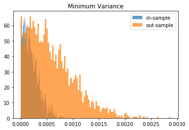
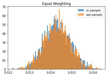
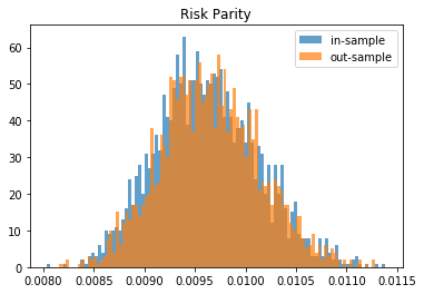
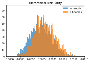
for method, distribs in empirical_volatilities.items():
    plt.hist(distribs['in-sample'], bins=100, label='in-sample', alpha=0.7)
    plt.hist(distribs['out-sample'], bins=100, label='out-sample', alpha=0.7)
    plt.title(method)
    plt.legend(loc=1)
    plt.show()
From this Monte Carlo study (it would benefit from more experiments), it stems that Hierarchical Risk Parity is rather stable, i.e. the distribution of the out-sample portfolio volatilities is rather similar to the distribution of the in-sample portfolio volatilities, only slightly shifted to the right (slightly higher volatility out-of-sample). On the contrary, distributions in-sample and out-sample of the Minimum Variance are wildly different despite being in a rather easy statistical regime for the estimation of the covariance matrix: N = 500 < T = 3 * 252. In this Monte Carlo study, Risk Parity performs well: very stable, and low out-sample portfolio volatility. However, it is very likely that the sampled correlation matrices do not verify the stylized facts of empirical financial correlations matrices which are:
-
large first eigenvalue
-
Perron-Frobenius property (dominant eigenvector with only positive entries)
-
significantly positive mean pairwise correlations
-
scale-free property of the minimum spanning tree of the correlation matrix (power-law type distribution of vertex degree)
-
hierarchical organization of the pairwise correlations (nested clusters of assets)
We can wonder how big is that subset in the set of all correlation matrices; likely very small. In that case, no wonder that the Hierarchical Risk Parity method does not perform at its best: It builds an order of the assets based on a hierarchical clustering algorithm whose result is totally spurious as no nested clusters exist. [TO BE VERIFIED / TESTED] In that specific case, using the bisection method (Lopez de Prado original algorithm implemented here) instead of following the dendrogram splits (an alternative idea which seems intuitively better) may alleviate the problem of finding a spurious correlation clustering hierarchy in the noise: Only the assets order is wrong; The successive (wrong) splits are discarded for the weights allocation.
The literature is for now short of a method to sample correlation matrices verifying the stylized properties (or at least, sampling correlation matrices very similar to the empirical ones). Another venue for research…