Hierarchical Risk Parity - Implementation & Experiments (Part III)
Hierarchical Risk Parity - Implementation & Experiments (Part III)
This blog follows Hierarchical Risk Parity - Implementation & Experiments (Part I) and Hierarchical Risk Parity - Implementation & Experiments (Part II).
In Part I, we implemented the ``Hierarchical Risk Parity’’ (HRP) approach proposed by Marcos Lopez de Prado in his paper Building Diversified Portfolios that Outperform Out-of-Sample and his book Advances in Financial Machine Learning.
In Part II, we compared the Hierarchical Risk Parity and standard naive approaches such as Equal Weighting, Risk Parity and Minimum Variance on in- and out-samples. Samples were generated from a centered multivariate Gaussian distribution parameterized by random correlation matrices (using an algorithm previously described in this blog post, which uniformly samples such matrices).
The goal of these simulations were to study the stability of the different methods between their in- and out-sample results. We found that HRP was relatively stable, but didn’t outperform a simple risk parity method (oblivious to any correlation structure). We concluded that this relative underperformance could come from the lack of hierarchical structure in the correlation matrices parameterizing the distribution from which samples were drawn.
So, about 1 year ago, I did the following remarks in the HRP blog Part II:
In a future experiment, we will try to sample correlation matrices which share common properties to the empirical ones estimated from financial correlations of assets or alphas.
[…]
However, it is very likely that the sampled correlation matrices do not verify the stylized facts of empirical financial correlations matrices which are:
large first eigenvalue
Perron-Frobenius property (dominant eigenvector with only positive entries)
significantly positive mean pairwise correlations
scale-free property of the minimum spanning tree of the correlation matrix (power-law type distribution of vertex degree)
hierarchical organization of the pairwise correlations (nested clusters of assets)
[…]
The literature is for now short of a method to sample correlation matrices verifying the stylized properties (or at least, sampling correlation matrices very similar to the empirical ones). Another venue for research…
I tackled this problem, and finally came up with a decent solution described in a few blog posts (by chronological order):
an arXiv preprint:
and a simple web app to visually and interactively showcase the output of the model:
TL;DR We find that the Hierarchical Risk Parity (HRP) is stable between the in-sample and out-sample (more stable than in the experiments described in HRP Part II which were using uniformly random and non-necessarily realistic correlation matrices); gives better results than the simple risk parity (which is oblivious to the correlation structure and cannot exploit it for better diversification), and the equal weighting (which is essentially the same as the risk parity as here, since using correlation matrices, all the volatilities are equal to 1 + estimation noise). The minimum variance doesn’t give stable solutions.
Sampling realistic financial correlation matrices using CorrGAN
As in HRP Part II, we will do a Monte Carlo study to compare the different allocation methods (equal weighting, minimum variance, risk parity, hierarchical risk parity). Unlike in HRP Part II, where we used uniformly random correlation matrices to parameterize the distribution from which we sampled the “returns”, we will use realistic yet synthetic correlation matrices generated from a Generative Adversarial Network (GAN) model.
In this section, as a first step, we will sample 2,000 correlation matrices using our CorrGAN model.
%matplotlib inline

import os
import glob
import imageio
import matplotlib.pyplot as plt
import pandas as pd
import numpy as np
import fastcluster
from scipy.cluster import hierarchy
from scipy.cluster.hierarchy import linkage
from scipy.spatial.distance import squareform
import PIL
import tensorflow as tf
from tensorflow.keras import layers
from statsmodels.stats.correlation_tools import corr_nearest
from tqdm import tqdm

from IPython import display
We define the architecture of the networks below:
def make_generator_model():
    model = tf.keras.Sequential()
    model.add(layers.Dense(25 * 25 * 256,
                           use_bias=False,
                           input_shape=(100,)))
    model.add(layers.BatchNormalization())
    model.add(layers.LeakyReLU())

    model.add(layers.Reshape((25, 25, 256)))
    assert model.output_shape == (None, 25, 25, 256)

    model.add(layers.Conv2DTranspose(128, (5, 5),
                                     strides=(1, 1),
                                     padding='same',
                                     use_bias=False))
    assert model.output_shape == (None, 25, 25, 128)
    model.add(layers.BatchNormalization())
    model.add(layers.LeakyReLU())

    model.add(layers.Conv2DTranspose(64, (5, 5),
                                     strides=(2, 2),
                                     padding='same',
                                     use_bias=False))
    assert model.output_shape == (None, 50, 50, 64)
    model.add(layers.BatchNormalization())
    model.add(layers.LeakyReLU())

    model.add(layers.Conv2DTranspose(1, (5, 5),
                                     strides=(2, 2),
                                     padding='same',
                                     use_bias=False,
                                     activation='tanh'))
    assert model.output_shape == (None, 100, 100, 1)

    return model
generator = make_generator_model()
def make_discriminator_model():
    model = tf.keras.Sequential()
    model.add(layers.Conv2D(64, (5, 5),
                            strides=(2, 2),
                            padding='same',
                            input_shape=[100, 100, 1]))
    model.add(layers.LeakyReLU())
    model.add(layers.Dropout(0.3))

    model.add(layers.Conv2D(128, (5, 5),
                            strides=(2, 2),
                            padding='same'))
    model.add(layers.LeakyReLU())
    model.add(layers.Dropout(0.3))

    model.add(layers.Flatten())
    model.add(layers.Dense(1))

    return model
discriminator = make_discriminator_model()
def discriminator_loss(real_output, fake_output):
    real_loss = cross_entropy(tf.ones_like(real_output),
                              real_output)
    fake_loss = cross_entropy(tf.zeros_like(fake_output),
                              fake_output)
    total_loss = real_loss + fake_loss
    return total_loss

def generator_loss(fake_output):
    return cross_entropy(tf.ones_like(fake_output),
                         fake_output)
generator_optimizer = tf.keras.optimizers.Adam(1e-4)
discriminator_optimizer = tf.keras.optimizers.Adam(1e-4)
We load the pre-trained weights (from the previous experiment described in this blog):
checkpoint_dir = './training_checkpoints'
checkpoint_prefix = os.path.join(checkpoint_dir, "ckpt")
checkpoint = tf.train.Checkpoint(generator_optimizer=generator_optimizer,
                                 discriminator_optimizer=discriminator_optimizer,
                                 generator=generator,
                                 discriminator=discriminator)
checkpoint.restore(tf.train.latest_checkpoint(checkpoint_dir))
Here, we sample noise from a 100 dimensional normal distribution, and feed these 2,000 random vectors to the GAN model in order to get the synthetic 2,000 correlation matrices:
n = 100
a, b = np.triu_indices(n, k=1)
MAX_COUNT = 2000

correl_mats = []
for count in range(MAX_COUNT):
    print(count)

    noise = tf.random.normal([1, 100])
    generated_image = generator(noise, training=False)

    correls = np.array(generated_image[0,:,:,0])
    # set diag to 1
    np.fill_diagonal(correls, 1)
    # symmetrize
    correls[b, a] = correls[a, b]
    # nearest corr
    nearest_correls = corr_nearest(correls)
    # set diag to 1
    np.fill_diagonal(nearest_correls, 1)
    # symmetrize
    nearest_correls[b, a] = nearest_correls[a, b]

    dist = 1 - nearest_correls
    Z = fastcluster.linkage(dist[a, b], method='ward')
    permutation = hierarchy.leaves_list(
        hierarchy.optimal_leaf_ordering(Z, dist[a, b]))
    prows = nearest_correls[permutation, :]
    ordered_corr = prows[:, permutation]

    correl_mats.append(ordered_corr)
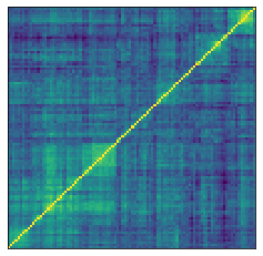
Below, we display one of the 2,000 synthetic correlation matrices generated by the GAN model:
plt.figure(figsize=(4, 4))
plt.pcolormesh(ordered_corr)

plt.tick_params(
    axis='both',
    which='both',
    bottom=False,
    top=False,
    left= False,
    labelbottom=False,
    labelleft=False)

plt.savefig('gan_matrices/correl_{}.png'.format(count),
            bbox_inches='tight',
            transparent=True)

plt.plot()
plt.show()
Definition of the weighting methods
Below, we define a couple of very simple ways of allocating capital to different assets, and the HRP method as described in Advances in Financial Machine Learning.
def compute_MV_weights(covariances):
    inv_covar = np.linalg.inv(covariances)
    u = np.ones(len(covariances))

    return np.dot(inv_covar, u) / np.dot(u, np.dot(inv_covar, u))


def compute_RP_weights(covariances):
    weights = (1 / np.diag(covariances))

    return weights / sum(weights)


def compute_unif_weights(covariances):

    return [1 / len(covariances) for i in range(len(covariances))]


def seriation(Z, N, cur_index):
    """Returns the order implied by a hierarchical tree (dendrogram).

       :param Z: A hierarchical tree (dendrogram).
       :param N: The number of points given to the clustering process.
       :param cur_index: The position in the tree for the recursive traversal.

       :return: The order implied by the hierarchical tree Z.
    """
    if cur_index < N:
        return [cur_index]
    else:
        left = int(Z[cur_index - N, 0])
        right = int(Z[cur_index - N, 1])
        return (seriation(Z, N, left) + seriation(Z, N, right))


def compute_serial_matrix(dist_mat, method="ward"):
    """Returns a sorted distance matrix.

       :param dist_mat: A distance matrix.
       :param method: A string in ["ward", "single", "average", "complete"].

        output:
            - seriated_dist is the input dist_mat,
              but with re-ordered rows and columns
              according to the seriation, i.e. the
              order implied by the hierarchical tree
            - res_order is the order implied by
              the hierarchical tree
            - res_linkage is the hierarchical tree (dendrogram)

        compute_serial_matrix transforms a distance matrix into
        a sorted distance matrix according to the order implied
        by the hierarchical tree (dendrogram)
    """
    N = len(dist_mat)
    flat_dist_mat = squareform(dist_mat)
    res_linkage = linkage(flat_dist_mat, method=method)
    res_order = seriation(res_linkage, N, N + N - 2)
    seriated_dist = np.zeros((N, N))
    a,b = np.triu_indices(N, k=1)
    seriated_dist[a,b] = dist_mat[[res_order[i] for i in a],
                                  [res_order[j] for j in b]]
    seriated_dist[b,a] = seriated_dist[a,b]

    return seriated_dist, res_order, res_linkage


def compute_HRP_weights(covariances):
    vols = np.sqrt(np.diag(covariances))
    correl_mat = np.multiply(covariances,
                         np.outer(vols**-1, vols**-1))
    # deal with precision errors
    np.fill_diagonal(correl_mat, 1)
    distances = np.sqrt((1 - correl_mat) / 2)
    # deal with precision errors
    np.fill_diagonal(distances, 0)
    ordered_dist_mat, res_order, res_linkage = compute_serial_matrix(
        distances, method='single')
    weights = pd.Series(1, index=res_order)
    clustered_alphas = [res_order]

    while len(clustered_alphas) > 0:
        clustered_alphas = [cluster[start:end] for cluster in clustered_alphas
                            for start, end in ((0, len(cluster) // 2),
                                               (len(cluster) // 2, len(cluster)))
                            if len(cluster) > 1]
        for subcluster in range(0, len(clustered_alphas), 2):
            left_cluster = clustered_alphas[subcluster]
            right_cluster = clustered_alphas[subcluster + 1]

            left_subcovar = covariances[left_cluster, :][:, left_cluster]
            inv_diag = 1 / np.diag(left_subcovar)
            parity_w = inv_diag * (1 / np.sum(inv_diag))
            left_cluster_var = np.dot(parity_w, np.dot(left_subcovar, parity_w))

            right_subcovar = covariances[right_cluster, :][:, right_cluster]
            inv_diag = 1 / np.diag(right_subcovar)
            parity_w = inv_diag * (1 / np.sum(inv_diag))
            right_cluster_var = np.dot(parity_w,
                                       np.dot(right_subcovar, parity_w))

            alloc_factor = 1 - left_cluster_var / (left_cluster_var +
                                                   right_cluster_var)

            weights[left_cluster] *= alloc_factor
            weights[right_cluster] *= 1 - alloc_factor

    return weights
Statistics in- and out-sample: portfolio volatility
To measure the performance of the methods, we will estimate the portfolio volatility in- and out-sample. They should be (approximately) the same, and as low as possible.
def compute_portfolio_volatility(weights, returns):
    return ((weights * returns)
            .sum(axis=1)
            .std() * np.sqrt(252))

def generate_returns_sample(covariances, horizon=252):
    return pd.DataFrame(
        np.random.multivariate_normal(
        np.zeros(len(covariances)), covariances,
        size=horizon))
We compute it below for one given synthetic correlation matrix:
cov_param = correl_mats[0]
in_sample = generate_returns_sample(cov_param, horizon=3 * 252)
out_sample = generate_returns_sample(cov_param, horizon=3 * 252)
methods = {
    'Minimum Variance': compute_MV_weights,
    'Risk Parity': compute_RP_weights,
    'Equal Weighting': compute_unif_weights,
    'Hierarchical Risk Parity': compute_HRP_weights,
}
for name, method in methods.items():
    in_sample_weights = method(in_sample.cov().values)

    in_sample_vol = compute_portfolio_volatility(
        in_sample_weights, in_sample)

    out_sample_vol = compute_portfolio_volatility(
        in_sample_weights, out_sample)

    print(name + ':\n' +
          'in-sample vol: ' + str(round(in_sample_vol, 4)) + '\n' +
          'out-sample vol: ' + str(round(out_sample_vol, 4)) +
          '\n\n')
Minimum Variance:
in-sample vol: 0.0
out-sample vol: 0.0


Risk Parity:
in-sample vol: 9.8106
out-sample vol: 10.2153


Equal Weighting:
in-sample vol: 9.8266
out-sample vol: 10.217


Hierarchical Risk Parity:
in-sample vol: 9.4994
out-sample vol: 9.9273
HRP gives better results than Risk Parity and Equal Weighting. Minimum Variance seems to give the best results on this instance.
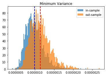
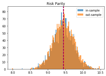
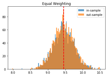
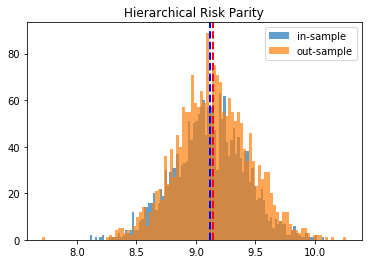
Monte Carlo study: Distribution of portfolio volatilities in-sample vs. out-sample
To have more confidence in the above results, we just repeat the experiment for the 2,000 matrices we have generated, and we plot the in- and out-sample distribution of portfolio volatilities. They should closely match, and have a mean as low as possible.
empirical_volatilities = {method: {'in-sample' : [], 'out-sample': []}
                          for method in methods.keys()}

nb_experiments = MAX_COUNT
idx = 0
for experiment in tqdm(range(nb_experiments)):
    true_covariances = correl_mats[idx]
    in_sample = generate_returns_sample(
        true_covariances, horizon=3 * 252)
    out_sample = generate_returns_sample(
        true_covariances, horizon=3 * 252)

    for name, method in methods.items():
        in_sample_weights = method(in_sample.cov().values)

        in_sample_vol = compute_portfolio_volatility(
            in_sample_weights, in_sample)

        out_sample_vol = compute_portfolio_volatility(
            in_sample_weights, out_sample)

        empirical_volatilities[name][
            'in-sample'].append(in_sample_vol)
        empirical_volatilities[name][
            'out-sample'].append(out_sample_vol)

    idx += 1
100%|██████████| 2000/2000 [15:19<00:00, 2.21it/s]
for method, distribs in empirical_volatilities.items():
    plt.hist(distribs['in-sample'], bins=100, label='in-sample', alpha=0.7)
    plt.hist(distribs['out-sample'], bins=100, label='out-sample', alpha=0.7)
    plt.axvline(x=np.mean(distribs['in-sample']), color='b',
                linestyle='dashed', linewidth=2)
    plt.axvline(x=np.mean(distribs['out-sample']), color='r',
                linestyle='dashed', linewidth=2)
    plt.title(method)
    plt.legend(loc=1)
    plt.show()
Conclusion: This blog post is a revamp of the HRP Part II study, but using this time more realistic correlation matrices to parameterize the “returns” distribution. With this more realistic assumption, we find this time that the HRP is clearly dominating the simple and naive risk parity allocation method. This is not surprising as the HRP, by design, encodes a stylized fact of the “returns” multivariate distribution: returns of assets are typically correlated in a hierarchical manner forming nested clusters describing coarsely the industries and broad industrial sectors up to the regional and global markets. Domain knowledge definitely helps design better Machine Learning algorithms.
What’s next? Can we further enhance this HRP algorithm by considering other stylized facts of the multivariate distribution of returns?