Comparison of Network-based and Minimum Variance Portfolios Using CorrGAN
Comparison of Network-based and Minimum Variance Portfolios Using CorrGAN
Many econophysicists have noticed that portfolios built using the leaves of networks built from an empirical correlation matrix estimated on the past returns of stocks (or other assets) are very similar to the portfolios obtained by applying a minimum variance optimization on the empirical covariance estimated on the same stocks.
the companies of the minimum risk Markowitz portfolio [MVP] are always located on the outer leaves of the [minimum spanning] tree’
– Onnela, J.-P., A. Chakraborti, K. Kaski, J. Kertész, and A. Kanto (2003). Dynamics of market correlations: Taxonomy and portfolio analysis. Phys. Rev. E 68(5), 056110
This recurring fact (the similarity of the portfolios obtained from these two different methods) have led researchers to think that there could be deep mathematical connections between the two methods.
In a very interesting paper, Hüttner et al. show that it is not the case.
Using Monte Carlo simulations, authors show that, in general, the solutions of the two portfolio construction methods can be very different: A Minimum Variance portfolio does not necessarily invest in the outer leaves of a network extracted from the same correlation matrix.
So, how to explain the empirical fact noticed by so many researchers?
Hüttner et al. suggest that it may come from special properties of the real empirical correlation matrices (as opposed to the uniformly random correlation matrices they used for the Monte Carlo simulations).
In their paper, they observe that:
the previous Monte Carlo studies should be rerun using simulation algorithms that are able to produce correlation matrices that display only a subset of these stylized facts, as opposed to completely random correlation matrices (which display none of them) and market correlation matrices (which exhibit them all). […] Concerning the generation of correlation matrices whose MSTs exhibit the scale-free property, to the best of our knowledge there is no algorithm available, and due to the generating mechanism of the MST we expect the task of finding such correlation matrices to be highly complex.
I have been mulling this problem for a while now, and I think that GANs could provide useful insights to this problem:
- GANs can help to sample realistic financial correlations (cf. CorrGAN),
- Exploring their latent space could provide a better understanding of the financial correlation matrices properties,
- Hopefully, disentangling the latent space could allow for controlling the generative model easily, and sample only correlation matrices verifying a subset of the stylized facts mentionned by Hüttner et al.
For now, we will only sample from CorrGAN (a GAN fitted on thousands of correlation matrices estimated from historical returns of S&P 500 stocks), and verify that Minimum Variance portfolios do indeed invest in the outer leaves of networks extracted from the same correlation matrices.
%matplotlib inline

import os
import numpy as np
import pandas as pd
import fastcluster
from scipy.cluster import hierarchy
from multiprocessing import Pool
from numpy.random import beta
from numpy.random import randn
from scipy.linalg import sqrtm
from numpy.random import seed
from tqdm import tqdm
import matplotlib.pyplot as plt


seed(42)
Let’s define two functions:
- compute the minimum variance weights
- compute the eigenvector centrality (one out of many definitions of centrality in networks)
def compute_mv_weights(C):
    ones = np.ones(len(C))
    inv_C = np.linalg.inv(C)

    return (np.dot(inv_C, ones) /
            np.dot(ones, np.dot(inv_C, ones)))

def compute_eigenvector_centrality(C):
    eigenvals, eigenvecs = np.linalg.eig(C)
    fst_eigenvec = eigenvecs[:, np.argmax(eigenvals)]

    return fst_eigenvec / np.sum(fst_eigenvec)
Totally random correlation matrices sampled using the onion method
The function below is useful to sample uniformly randomly correlation matrices in the elliptope according to the onion method.
def sample_unif_correlmat(dimension):
    d = dimension + 1

    prev_corr = np.matrix(np.ones(1))
    for k in range(2, d):
        # sample y = r^2 from a beta distribution
        # with alpha_1 = (k-1)/2 and alpha_2 = (d-k)/2
        y = beta((k - 1) / 2, (d - k) / 2)
        r = np.sqrt(y)

        # sample a unit vector theta uniformly
        # from the unit ball surface B^(k-1)
        v = randn(k-1)
        theta = v / np.linalg.norm(v)

        # set w = r theta
        w = np.dot(r, theta)

        # set q = prev_corr**(1/2) w
        q = np.dot(sqrtm(prev_corr), w)

        next_corr = np.zeros((k, k))
        next_corr[:(k-1), :(k-1)] = prev_corr
        next_corr[k-1, k-1] = 1
        next_corr[k-1, :(k-1)] = q
        next_corr[:(k-1), k-1] = q

        prev_corr = next_corr

    return prev_corr
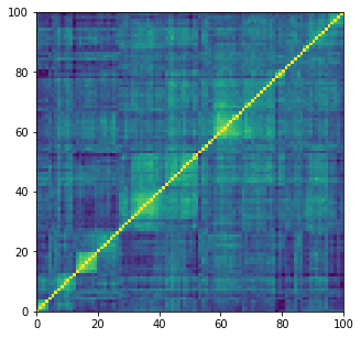
Realistic financial correlation matrices generated from CorrGAN
Let’s load 10,000 correlation matrices of size 100 x 100 which were previously generated by CorrGAN.
n = 100
a, b = np.triu_indices(n, k=1)

gan_corrs = []
for r, d, files in os.walk('gan_corrs/'):
    for file in files:
        flat_corr = np.load('gan_corrs/{}'.format(file))
        corr = np.ones((n, n))
        corr[a, b] = flat_corr
        corr[b, a] = flat_corr
        gan_corrs.append(corr)
plt.figure(figsize=(5, 5))
plt.pcolormesh(gan_corrs[0])
plt.show()
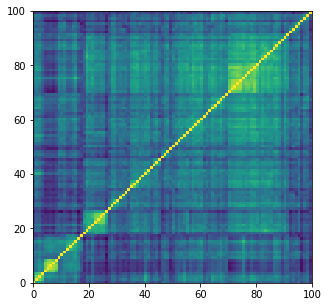
Load empirical correlation matrices estimated from S&P 500 stocks
real_corrs = []
for r, d, files in os.walk('corrs_med/'):
    for file in files:
        if 'corr_emp_100d_batch' in file:
            flat_corr = pd.read_hdf('corrs_med/{}'.format(file))
            corr = np.ones((n, n))
            corr[a, b] = flat_corr
            corr[b, a] = flat_corr
            real_corrs.append(corr)

        if len(real_corrs) >= 10000:
            break
dist = 1 - real_corrs[0]
Z = fastcluster.linkage(dist[a, b], method='ward')
permutation = hierarchy.leaves_list(
    hierarchy.optimal_leaf_ordering(Z, dist[a, b]))
prows = real_corrs[0][permutation, :]
ordered_corr = prows[:, permutation]

plt.figure(figsize=(5, 5))
plt.pcolormesh(ordered_corr)
plt.show()
MVP and eigenvector centrality
The statistics defined below is used to measure to which extent the MVP is investing in the outer leaves of the network:
(portfolio weight of the 20% least central assets) / 0.2
If, in average, this statistic is equal to 1, it means that there is no relation between the MVP and eigenvector centrality. If significantly below 1, then the MVP is investing in central assets. If well above 1, then the MVP is investing in the leaves.
def compute_stat_1(C, p=0.2):
    MVP_weights = compute_mv_weights(C)
    centralities = compute_eigenvector_centrality(C)
    # find the k (20%) smallest values
    k = int(len(C) * p)
    idx = centralities.argsort()[:k]

    return MVP_weights[idx].sum() / p
Monte Carlo simulations
nb_samples = len(gan_corrs)
list_nb_assets = [gan_corrs[0].shape[0]]

unif_ratios = {}
gan_ratios = {}
real_ratios = {}
for nb_assets in list_nb_assets:
    correlmats = [sample_unif_correlmat(nb_assets)
                  for sample in tqdm(range(nb_samples))]

    with Pool() as pool:
        values = list(
            tqdm(pool.imap_unordered(compute_stat_1,
                                     correlmats),
                 total=nb_samples))

    unif_ratios[nb_assets] = values

    with Pool() as pool:
        values = list(
            tqdm(pool.imap_unordered(compute_stat_1,
                                     gan_corrs),
                 total=nb_samples))

    gan_ratios[nb_assets] = values

    with Pool() as pool:
        values = list(
            tqdm(pool.imap_unordered(compute_stat_1,
                                     real_corrs),
                 total=nb_samples))

    real_ratios[nb_assets] = values
for d in list_nb_assets:
    unif_density, unif_edges, unif_hist = plt.hist(
        unif_ratios[d], bins=10000, density=True,
        stacked=True)
    unif_proba = sum([v for (v, b) in zip(unif_density, unif_edges)
                      if b <= 1]) * (unif_edges[1] - unif_edges[0])
    plt.clf()
    gan_density, gan_edges, gan_hist = plt.hist(
        gan_ratios[d], bins=10000, density=True,
        stacked=True)
    gan_proba = sum([v for (v, b) in zip(gan_density, gan_edges)
                     if b <= 1]) * (gan_edges[1] - gan_edges[0])
    plt.clf()
    real_density, real_edges, real_hist = plt.hist(
        real_ratios[d], bins=10000, density=True,
        stacked=True)
    real_proba = sum([v for (v, b) in zip(real_density, real_edges)
                      if b <= 1]) * (real_edges[1] - real_edges[0])
    plt.clf()

    plt.figure(figsize=(15, 10))
    plt.title(r'$\dfrac{portfolio~weight~of~the~20\%~least~central~assets}{0.2}$'
              + "\tfor correlation matrices with shape $100 \\times 100$",
              fontsize=16)
    bins = np.linspace(-6, 20, 100)

    # uniform random correlation matrices
    plt.hist(unif_ratios[d], bins, alpha=0.8,
             label="(unif correl mats) mean = "
             + str(round(np.mean(unif_ratios[d]), 2))
             + ", proba(stat < 1) = " + str(round(np.mean(unif_proba), 2)))
    plt.axvline(x=np.mean(unif_ratios[d]),
                color='b', linestyle='dashed', linewidth=2)

    # real financial correlation matrices
    plt.hist(real_ratios[d], bins, alpha=0.8,
             label="(real correl mats) mean = "
             + str(round(np.mean(real_ratios[d]), 2))
             + ", proba(stat < 1) = " + str(round(np.mean(real_proba), 2)))
    plt.axvline(x=np.mean(real_ratios[d]),
                color='r', linestyle='dashed', linewidth=2)

    # realistic random correlation matrices generated by CorrGAN
    plt.hist(gan_ratios[d], bins, alpha=0.8,
             label="(gan correl mats) mean = "
             + str(round(np.mean(gan_ratios[d]), 2))
             + ", proba(stat < 1) = " + str(round(np.mean(gan_proba), 2)))
    plt.axvline(x=np.mean(gan_ratios[d]),
                color='g', linestyle='dashed', linewidth=2)

    # baseline: 1 means no relation between centrality and MV weights
    plt.axvline(x=1, color='k', linestyle='dashed', linewidth=2)

    plt.legend()
    plt.show()
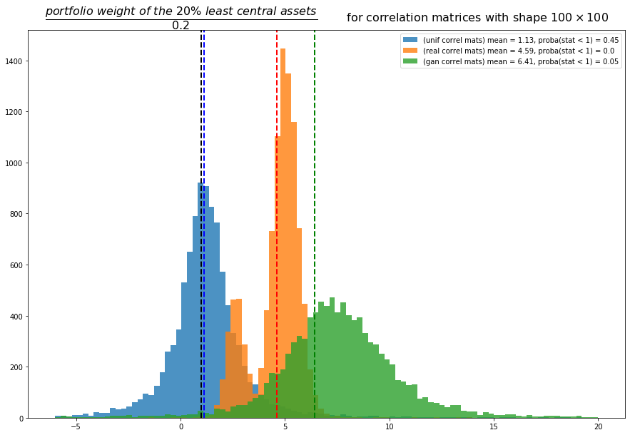
Conclusion: Not a very conclusive conclusion. This study brings more questions…
First, we can reproduce the results from Hüttner et al. using uniformly random correlation matrices: In general, there is no relation between minimum variance portfolios and centrality (blue distribution).
However, for real correlation matrices estimated from market returns (orange distribution), we can notice that the mean of the statistic is significantly above 1, and even stronger, there are no values below 1, confirming the remarks from empirical researchers: Markowitz / Minimum Variance Portfolios (MVPs) tend to invest in leaves of correlation networks. All the MVPs portfolios built from the real correlations overweight the assets located at the leaves of the networks. Why is the statistic distribution bimodal? Could it be because there are essentially two types of correlation matrices, and MVP behaviours? For example, stressed market periods vs. normal market periods. In stressed periods where correlation is high in general (approximately one factor), the correlation network would take a star topology (imagine one central asset and many leaves connected directly to this central asset). In this start toplogy configuration, the many leaves would receive an approximately equal allocation, and therefore the 20% least central assets wouldn’t overweight by much the 20% baseline. Whereas in normal conditions where more diverse factors of risk drive the assets, the correlation network topology would contain deeper and much less correlated leaves which would get much more allocation from the MVP and therefore overweighting by a wider magin the baseline of 20% allocation. This hypothesis has to be investigated further.
Concerning the correlation matrices generated by CorrGAN, they also show that, in practice, for realistic financial correlations, MVP and network-based portfolios tend to select the same assets. Only 5% of all the portfolios don’t overweight the 20% least central assets. But, otherwise, these 20% least central assets are even more overweighted than using the real empirical correlation matrices. We can see here that the GAN has not captured perfectly all the properties of the empirical matrices: The statistic derived to compare MVP and network-based portfolios doesn’t have a bimodal distribution when we use the synthetic matrices. Did the GAN failed to capture modes of the empirical distribution of financial correlation matrices? Correlations of stressed periods vs. normal periods? Need to investigate further using a cGAN fitting on stressed and normal periods. Any difference? Do we capture the bimodal distribution of this MVP centrality statistic?