S&P 500 Sharpe vs. Correlation Matrices - Building a dataset for generating stressed/rally/normal scenarios
S&P 500 Sharpe vs. Correlation Matrices - Building a dataset for generating stressed/rally/normal scenarios
In this blog, we just do basic data exploration. The goal is to build a dataset containing 3 classes of $100 \times 100$ correlation matrices:
- correlation matrices associated to a stressed market,
- correlation matrices associated to a rally market,
- correlation matrices associated to a normal market.
The following definitions are somewhat arbitrary (and could be changed):
Definition of ‘stressed market’: A market is ‘stressed’ whenever the equi-weighted basket of 100 stocks under consideration has a Sharpe below -0.5 over the year of study (252 trading days).
Definition of ‘rally market’: A market is ‘rallying’ whenever the equi-weighted basket of 100 stocks under consideration has a Sharpe above 2 over the year of study (252 trading days).
Definition of ‘normal market’: A market is ‘normal’ whenever the equi-weighted basket of 100 stocks under consideration has a Sharpe in-between -0.5 and 2 over the year of study (252 trading days).
Once we get this dataset, we can fit generative models such as conditional CorrGAN or conditional CorrVAE (ongoing research) to generate unseen correlation matrices that look like real ones. With these generative models, we can then compare the performance of different risk-based portfolio construction methods such as the Hierarchical Risk Parity, the Hierarchical Equal Risk Contribution, risk parity, inverse volatility, minimum variance, equal weighting, etc. on simulated but not too unrealistic data. Obviously, any conclusion is dependent on the simulated data and ultimately on the generative models, and might not generalize to real data, but these Monte Carlo experiments yield to a better understanding of (the numerical behaviour of) these methods than applying and comparing them directly on a cherry-picked real dataset (arbitrary period and choice of assets).
TL;DR Not much. Just a script to generate 3 classes of correlation matrices for further studies (conditional GANs and VAEs). Brief study of mean correlation and correlation coefficient distributions vs. Sharpe and market ‘state’ (stressed/rally/normal). Nearly mechanically, there is an anti-correlation between Sharpe and mean correlation of the 100 equi-weighted stocks: Everything else being equal, when mean correlation is high, variance of the basket tends to be higher, and therefore Sharpe tends to be lower; Conversely, when mean correlation is low, variance of the basket tends to be lower, and therefore Sharpe tends to be higher. However, this is not always the case that high mean correlation is associated with low Sharpe and conversely (transition between regime?).
import sys
from random import randint
import pandas as pd
import numpy as np
import fastcluster
from scipy.cluster import hierarchy
from scipy.stats import rankdata
import matplotlib.pyplot as plt
from mpl_toolkits.mplot3d import Axes3D
import matplotlib.pyplot as plt
Read a file downloaded from Quandl (3 years ago) containing adjusted (for corporate actions such as stock splits, dividends, etc.) prices for S&P 500 constituents from 2000 to 2016.
df = pd.read_csv('data/SP500_HistoTimeSeries.csv')

df['Date'] = pd.to_datetime(df['Date'], infer_datetime_format=True)

df.index = df['Date']
del df['Date']
df = df.sort_index()

returns = df.pct_change(periods=1)
dim = 100
tri_a, tri_b = np.triu_indices(dim, k=1)
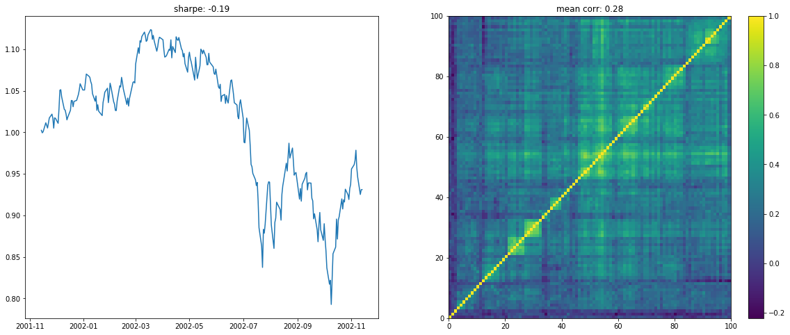
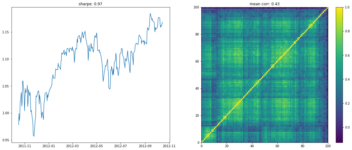
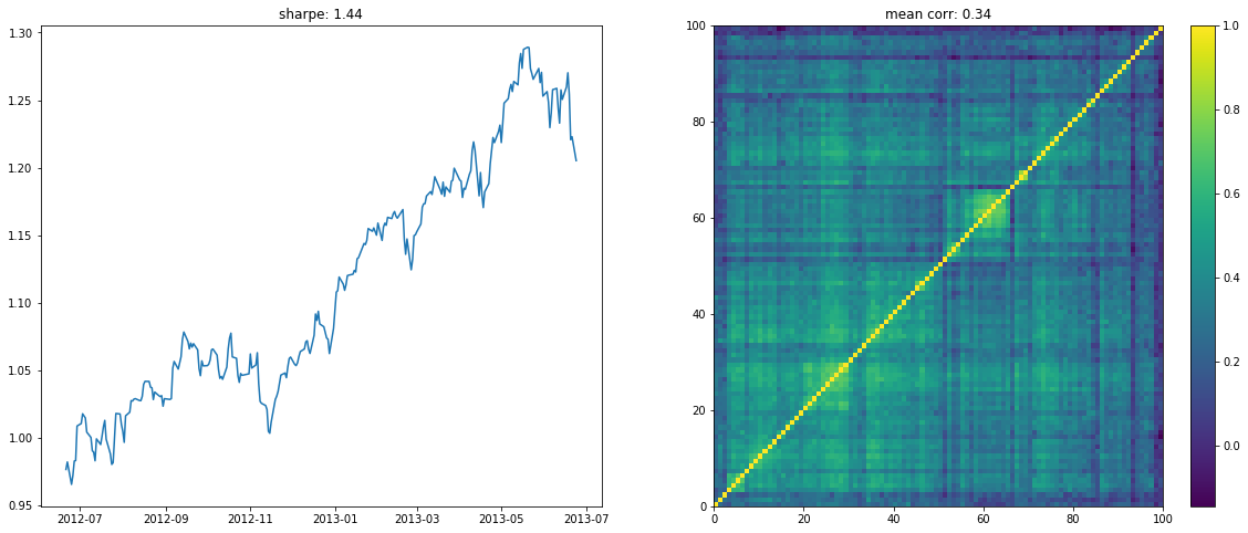
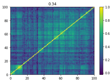
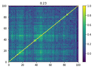
Sample at random a year of daily returns (252 consecutive trading days) for all the 500 stocks. Discard the stocks with missing values. Choose at random 100 stocks amongst the ones still available (having full history for that year). Estimate the $100 \times 100$ empirical correlation matrix. Depending on the Sharpe of the equi-weighted basket of these 100 stocks that particular year, assign this matrix one of the 3 classes: stressed (Sharpe below -0.5), rally (Sharpe above 2), normal (Sharpe in-between -0.5 and 2).
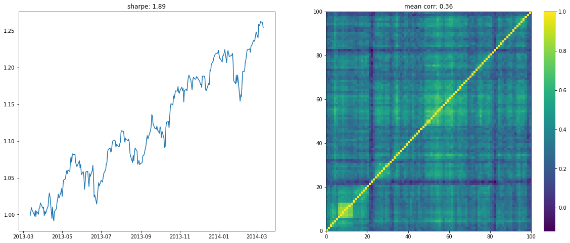
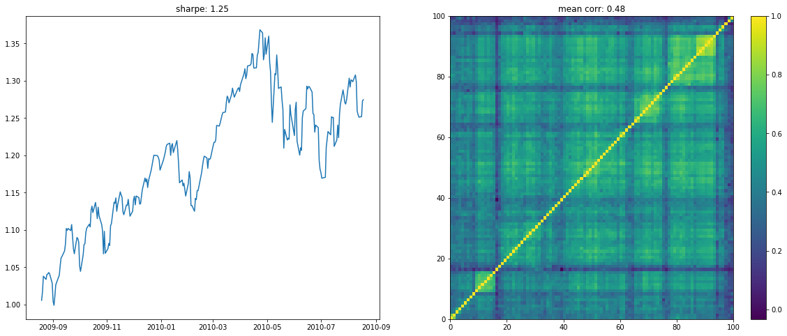
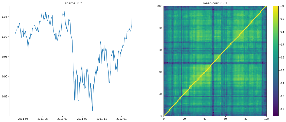
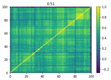
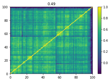
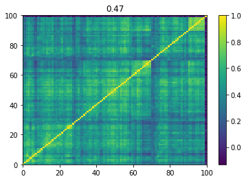
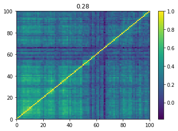
We display below a few of such re-ordered correlation matrices alongside the performance of the associated equi-weighted basket for that year.
corr_vs_sharpe = []
stressed_mats = []
stressed_count = 0
rally_mats = []
rally_count = 0
normal_mats = []
normal_count = 0
for loop in range(20000):
    try:
        t_idx = randint(0, len(returns) - 252)

        period_returns = returns.iloc[t_idx:(t_idx + 252)]

        rmv = 0
        for col in period_returns.columns:
            if len(period_returns[col].dropna()) < 252:
                rmv += 1
                del period_returns[col]
        rmv, period_returns.shape

        idx = list(np.random.choice(len(period_returns.columns), dim,
                                    replace=False))

        period_returns[period_returns.columns[idx]].dropna().shape

        corr = period_returns[
            period_returns.columns[idx]].dropna().corr().values
        corr.mean()

        mean_return = (period_returns[period_returns.columns[idx]]
                       .dropna()
                       .mean(axis=1)
                       .mean() * 252)
        vol = (period_returns[period_returns.columns[idx]]
               .dropna()
               .mean(axis=1)
               .std() * np.sqrt(252))
        sharpe = mean_return / vol

        dist = 1 - corr
        Z = fastcluster.linkage(dist[tri_a, tri_b], method='ward')
        permutation = hierarchy.leaves_list(
            hierarchy.optimal_leaf_ordering(Z, dist[tri_a, tri_b]))
        prows = corr[permutation, :]
        ordered_corr = prows[:, permutation]

        corr_vs_sharpe.append([corr.mean(), sharpe])

        if sharpe < -0.5:
            stressed_mats.append(ordered_corr)
            np.save('stressed_mats/mat_{}.npy'.format(stressed_count),
                    ordered_corr)
            stressed_count += 1
        elif sharpe > 2:
            rally_mats.append(ordered_corr)
            np.save('rally_mats/mat_{}.npy'.format(rally_count),
                    ordered_corr)
            rally_count += 1
        else:
            normal_mats.append(ordered_corr)
            np.save('normal_mats/mat_{}.npy'.format(normal_count),
                    ordered_corr)
            normal_count += 1

        if loop < 10:
            plt.figure(figsize=(20, 8))
            plt.subplot(1, 2, 1)
            plt.plot((1 + period_returns[
                period_returns.columns[idx]]
                      .dropna().mean(axis=1)).cumprod())
            plt.title("sharpe: " + str(np.round(sharpe, 2)))

            plt.subplot(1, 2, 2)
            plt.pcolormesh(ordered_corr)
            plt.colorbar()
            plt.title("mean corr: " + str(np.round(corr.mean(), 2)))
            plt.show()
    except:
        pass
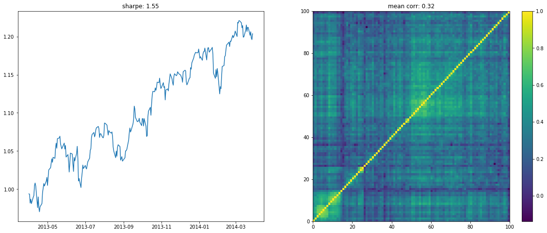
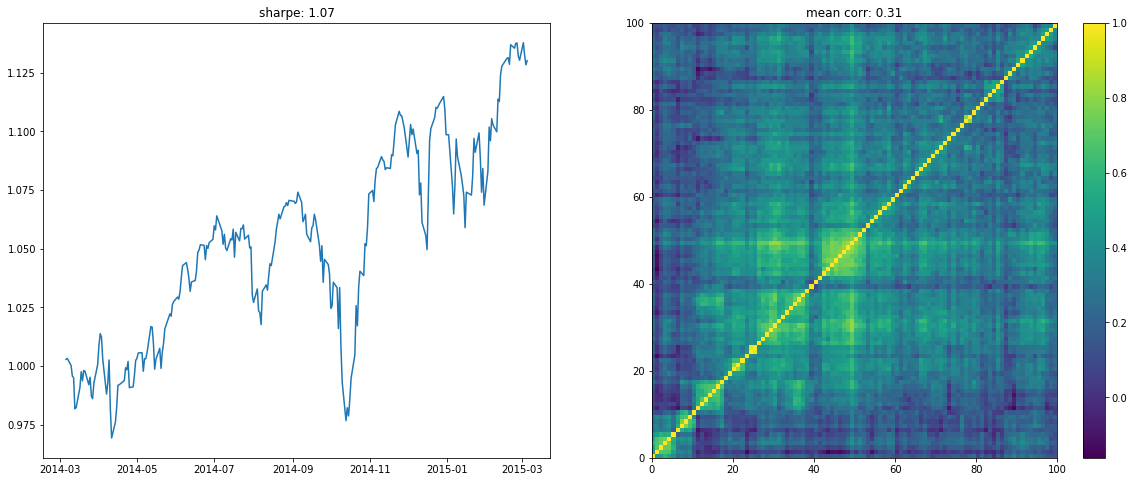
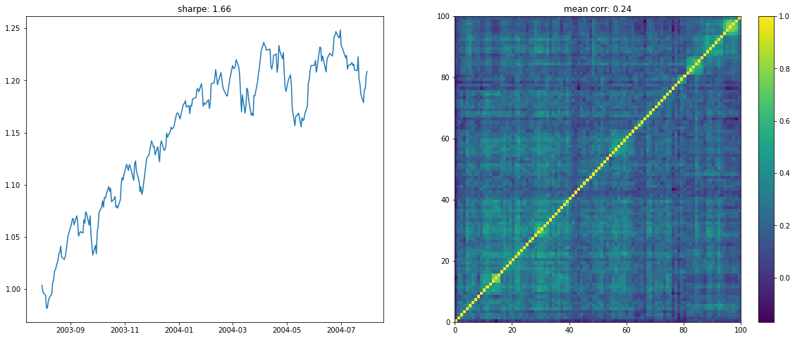
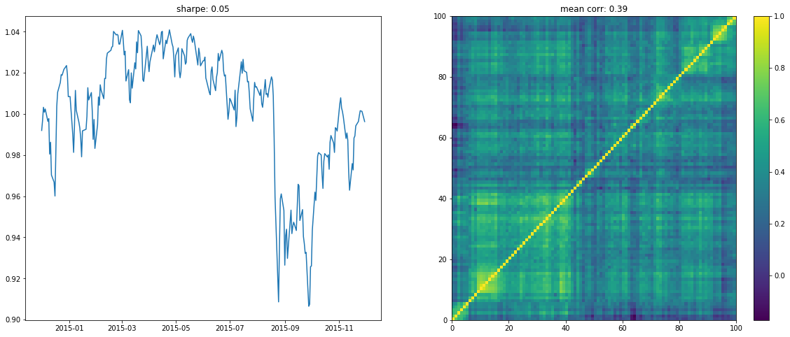
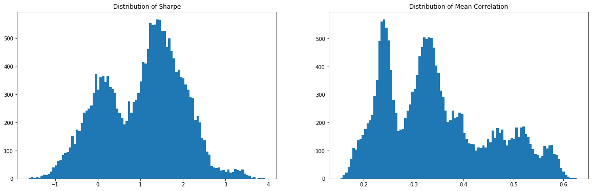
On the left the distribution of the Sharpe values (one Sharpe value per sample of 1 year x 100 stocks chosen). We can observe essentially two modes: one mode at 0, and another one at around 1.5 with twice as much samples. Concerning the mean correlation values (one mean correlation value per sample of 1 year x 100 stocks chosen), we can observe several modes:
- at 0.25 (low correlation regime),
- at 0.34 (average typical correlation),
- around 0.5 (high correlation regime typical of stressed markets).
corr_vs_sharpe = np.array(corr_vs_sharpe)

plt.figure(figsize=(20, 6))
plt.subplot(1, 2, 1)
plt.hist(corr_vs_sharpe[:, 1], bins=100)
plt.title('Distribution of Sharpe')

plt.subplot(1, 2, 2)
plt.hist(corr_vs_sharpe[:, 0], bins=100)
plt.title('Distribution of Mean Correlation')
plt.show()
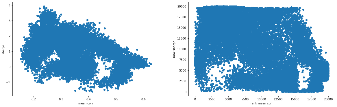
We illustrate the anti-correlation relationship between Sharpe and mean correlation in the following graph: High mean correlation tends to be associated with low Sharpe; Low mean correlation tends to be associated with high Sharpe. The relation is not perfect as you can see below, part of it might be due to regime transition?
plt.figure(figsize=(20, 6))
plt.subplot(1, 2, 1)
plt.scatter(corr_vs_sharpe[:, 0], corr_vs_sharpe[:, 1])
plt.xlabel('mean corr')
plt.ylabel('sharpe')

plt.subplot(1, 2, 2)
plt.scatter(rankdata(corr_vs_sharpe[:, 0]),
            rankdata(corr_vs_sharpe[:, 1]))
plt.xlabel('rank mean corr')
plt.ylabel('rank sharpe')
plt.show()
From this sampling procedure, out of 20000 matrices we obtain the following:
len(stressed_mats), len(rally_mats), len(normal_mats)
(1004, 3091, 15897)
That is, 5% of stressed matrices, 15% of rally matrices, 80% of normal matrices.
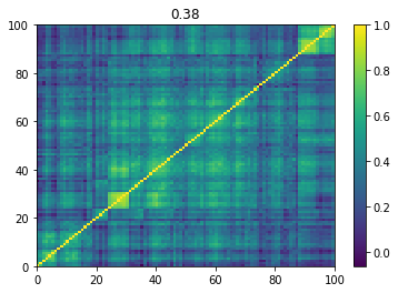
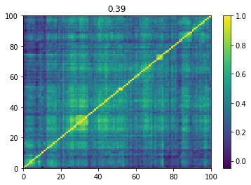
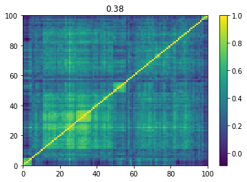
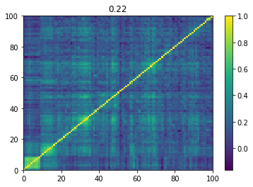
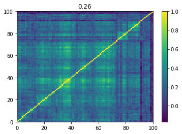
Below we displayed a few re-ordered correlation matrices which are associated to the ‘stressed’ market state.
for i, mat in enumerate(stressed_mats):
    plt.pcolormesh(mat)
    plt.colorbar()
    plt.title(round(mat.mean(), 2))
    plt.show()

    if i > 5:
        break
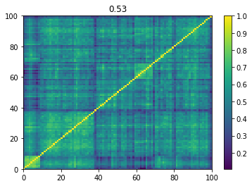
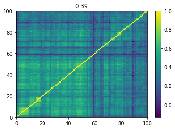
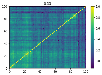
Below we displayed a few re-ordered correlation matrices which are associated to the ‘rally’ market state.
for i, mat in enumerate(rally_mats):
    plt.pcolormesh(mat)
    plt.colorbar()
    plt.title(round(mat.mean(), 2))
    plt.show()

    if i > 5:
        break
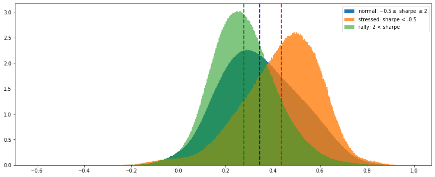
And, finally, we display the distributions of all the correlation coefficients from all the matrices associated to the 3 market states (stressed in orange, rally in green, normal in blue):
stressed_corr_coeffs = []
for mat in stressed_mats:
    stressed_corr_coeffs.extend(list(mat[tri_a, tri_b]))

rally_corr_coeffs = []
for mat in rally_mats:
    rally_corr_coeffs.extend(list(mat[tri_a, tri_b]))

normal_corr_coeffs = []
for mat in normal_mats:
    normal_corr_coeffs.extend(list(mat[tri_a, tri_b]))
nbins = 500
plt.figure(figsize=(15, 6))
plt.hist(normal_corr_coeffs, bins=nbins, alpha=1,
         label='normal: $-0.5 \leq$ sharpe $\leq 2$',
         density=True, log=False)
plt.axvline(x=np.mean(normal_corr_coeffs), color='b',
            linestyle='dashed', linewidth=2)
plt.hist(stressed_corr_coeffs, bins=nbins, alpha=0.8,
         label='stressed: sharpe < -0.5',
         density=True, log=False)
plt.axvline(x=np.mean(stressed_corr_coeffs), color='r',
            linestyle='dashed', linewidth=2)
plt.hist(rally_corr_coeffs, bins=nbins, alpha=0.6,
         label='rally: 2 < sharpe',
         density=True, log=False)
plt.axvline(x=np.mean(rally_corr_coeffs), color='g',
            linestyle='dashed', linewidth=2)
plt.legend()
plt.show()
We observe that correlation matrices associated to a stressed market have much higher correlation coefficients (with a mode at 0.55). The distribution of rally matrices is the most symmetric (with a mode at around 0.25).
Conclusion: In this blog, we illustrated the (rather contemporaneous) relation between correlation and Sharpe (note that this relation can be justified by investors’ herding/rushing behaviour in extreme markets, but also ‘mechanically’ as volatility of a portfolio is tied to correlation of its assets). Mainly, this blog purpose is to illustrate the sampling process that I use in order to build a training database for fitting conditional (to a market state) GANs and VAEs. I aim to have 20000 samples of each classes before trying to fit the conditional GAN/VAE models. Then, hopefully, I will be able to horse-race portfolio construction methods on different market states thanks to the conditional GAN/VAE, and gain a better understanding of their behaviour and performance.