CorrVAE: A VAE for sampling realistic financial correlation matrices (Tentative I)
CorrVAE: A VAE for sampling realistic financial correlation matrices (Tentative I)
First tentative at CorrVAE. Work in progress. Basically, inspired from the following tutorial:
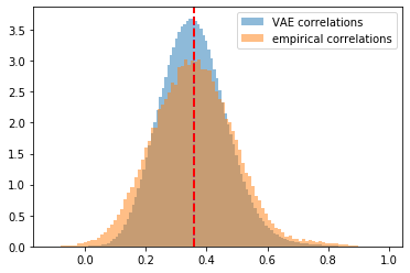
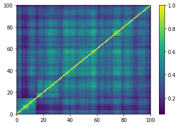
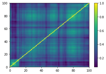
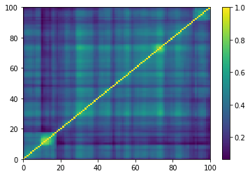
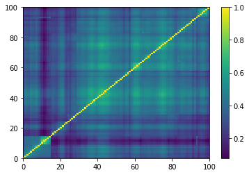
However, the tutorial assumes that each pixel follows a Bernoulli distribution whereas correlation matrix coefficients live in [-1, 1]. Applying very naively the tutorial gives the following results. They are not too bad as S&P 500 stocks empirical correlations are mostly positive (cf. these stylized facts), and symmetrically centered around a mean of 0.4 approximately. It happens that the for this distribution the loss “reconstruction loss + Kullback–Leibler loss” is well balanced, and behaves nicely.
If one tries to pre-process the correlation matrix to normalize its coefficients within [0, 1] using, for example, $f: \rho \mapsto (1 + \rho) / 2$, then naively apply the above tutorial, and finally un-normalize the coefficients into the orignal range [-1, 1] using, for example, $f^{-1}: x \mapsto 2x - 1$, results happen to be very poor as the Kullback-Leibler loss (the regularization part) becomes too important in the overall loss: Results obtained are more or less an average of the dataset (too much regularization). I tried to use some “annealing”, that is, start training with the reconstruction loss only, and then adding the Kullback-Leibler loss progressively, without great success. As of now, I’m obtaining my best results by balancing reconstruction loss R and Kullback-Leibler loss KL in such an ad hoc way: R + 0.05 KL.
To be continued…
import os
import time
import numpy as np
import pandas as pd
import tensorflow as tf
import glob
import matplotlib.pyplot as plt
import PIL
import imageio

from IPython import display

%matplotlib inline
n = 100
a, b = np.triu_indices(n, k=1)

corrs = []
for r, d, files in os.walk('sorted_corrs_med/'):
    for file in files:
        if 'corr_emp_{}d_batch_'.format(n) in file:
            flat_corr = pd.read_hdf('sorted_corrs_med/{}'.format(file))
            corr = np.ones((n, n))
            corr[a, b] = flat_corr
            corr[b, a] = flat_corr
            corrs.append(corr)
corrs = np.array(corrs)
plt.figure(figsize=(5, 5))
plt.pcolormesh(corrs[0])
plt.show()
train_size = 14000
train_images = corrs[:train_size]
test_images = corrs[train_size:]
train_images = train_images.reshape(
    train_images.shape[0], n, n, 1).astype('float32')
test_images = test_images.reshape(
    test_images.shape[0], n, n, 1).astype('float32')
TRAIN_BUF = train_size
TEST_BUF = len(corrs) - train_size
BATCH_SIZE = 100
train_dataset = (tf.data.Dataset
                 .from_tensor_slices(train_images)
                 .shuffle(TRAIN_BUF)
                 .batch(BATCH_SIZE))
test_dataset = (tf.data.Dataset
                .from_tensor_slices(test_images)
                .shuffle(TEST_BUF)
                .batch(BATCH_SIZE))
class CVAE(tf.keras.Model):
    def __init__(self, latent_dim):
        super(CVAE, self).__init__()
        self.latent_dim = latent_dim
        self.inference_net = tf.keras.Sequential([
            tf.keras.layers.InputLayer(input_shape=(n, n, 1)),
            tf.keras.layers.Conv2D(
                filters=32, kernel_size=3, strides=(2, 2), activation='relu'),
            tf.keras.layers.Conv2D(
                filters=64, kernel_size=3, strides=(2, 2), activation='relu'),
            tf.keras.layers.Conv2D(
                filters=128, kernel_size=3, strides=(2, 2), activation='relu'),
            tf.keras.layers.Flatten(),
            # No activation
            tf.keras.layers.Dense(latent_dim + latent_dim),
        ])

        self.generative_net = tf.keras.Sequential([
            tf.keras.layers.InputLayer(input_shape=(latent_dim,)),
            tf.keras.layers.Dense(units=25*25*64, activation=tf.nn.relu),
            tf.keras.layers.Reshape(target_shape=(25, 25, 64)),
            tf.keras.layers.Conv2DTranspose(
                filters=128,
                kernel_size=3,
                strides=(1, 1),
                padding="SAME",
                activation='relu'),
            tf.keras.layers.Conv2DTranspose(
                filters=64,
                kernel_size=3,
                strides=(2, 2),
                padding="SAME",
                activation='relu'),
            tf.keras.layers.Conv2DTranspose(
                filters=32,
                kernel_size=3,
                strides=(2, 2),
                padding="SAME",
                activation='relu'),
            # No activation
            tf.keras.layers.Conv2DTranspose(
                filters=1,
                kernel_size=3,
                strides=(1, 1),
                padding="SAME"),
        ])

    @tf.function
    def sample(self, eps=None):
        if eps is None:
            eps = tf.random.normal(shape=(BATCH_SIZE, self.latent_dim))
        return self.decode(eps, apply_sigmoid=True)

    def encode(self, x):
        mean, logvar = tf.split(self.inference_net(x),
                                num_or_size_splits=2, axis=1)
        return mean, logvar

    def reparameterize(self, mean, logvar):
        eps = tf.random.normal(shape=mean.shape)
        return eps * tf.exp(logvar * .5) + mean

    def decode(self, z, apply_sigmoid=False):
        logits = self.generative_net(z)
        if apply_sigmoid:
            probs = tf.sigmoid(logits)
            return probs

        return logits
optimizer = tf.keras.optimizers.Adam(1e-4)

def log_normal_pdf(sample, mean, logvar, raxis=1):
    log2pi = tf.math.log(2. * np.pi)
    return tf.reduce_sum(
        -.5 * ((sample - mean) ** 2. * tf.exp(-logvar) + logvar + log2pi),
        axis=raxis)

@tf.function
def compute_loss(model, x):
    mean, logvar = model.encode(x)
    z = model.reparameterize(mean, logvar)
    x_logit = model.decode(z)

    cross_ent = tf.nn.sigmoid_cross_entropy_with_logits(logits=x_logit,
                                                        labels=x)
    logpx_z = -tf.reduce_sum(cross_ent, axis=[1, 2, 3])
    logpz = log_normal_pdf(z, 0., 0.)
    logqz_x = log_normal_pdf(z, mean, logvar)
    return -tf.reduce_mean(logpx_z + logpz - logqz_x)

@tf.function
def compute_apply_gradients(model, x, optimizer):
    with tf.GradientTape() as tape:
        loss = compute_loss(model, x)
    gradients = tape.gradient(loss, model.trainable_variables)
    optimizer.apply_gradients(zip(gradients, model.trainable_variables))
epochs = 1000
latent_dim = 100
num_examples_to_generate = 16

random_vector_for_generation = tf.random.normal(
    shape=[num_examples_to_generate, latent_dim])
model = CVAE(latent_dim)
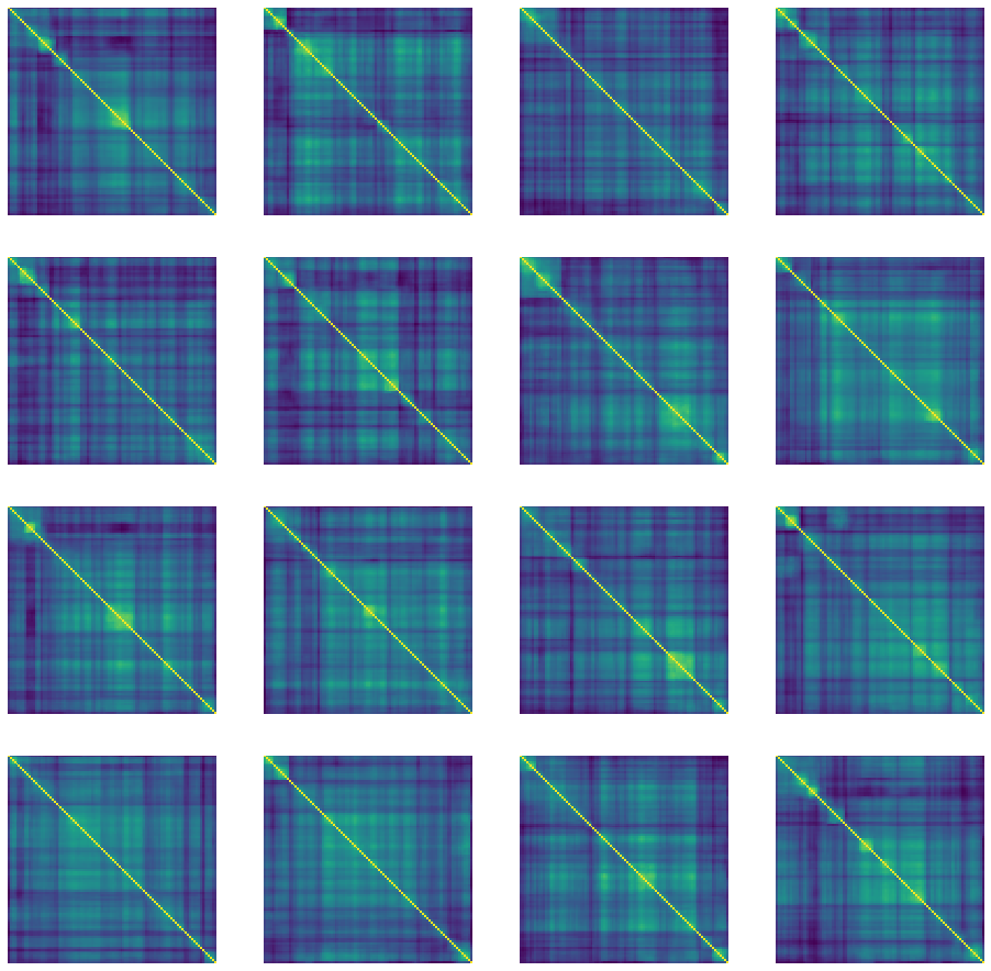
def generate_and_save_images(model, epoch, test_input):
    predictions = model.sample(test_input)
    fig = plt.figure(figsize=(16, 16))

    for i in range(predictions.shape[0]):
        plt.subplot(4, 4, i+1)
        plt.imshow(predictions[i, :, :, 0])
        plt.axis('off')

    plt.savefig('image_at_epoch_{:04d}.png'.format(epoch))
    plt.show()
generate_and_save_images(model, 0, random_vector_for_generation)

for epoch in range(1, epochs + 1):
    start_time = time.time()
    for train_x in train_dataset:
        compute_apply_gradients(model, train_x, optimizer)
    end_time = time.time()

    if epoch % 1 == 0:
        loss = tf.keras.metrics.Mean()
        for test_x in test_dataset:
            loss(compute_loss(model, test_x))
        elbo = -loss.result()
        display.clear_output(wait=False)
        print('Epoch: {}, Test set ELBO: {}, '
              'time elapse for current epoch {}'.format(epoch,
                                                        elbo,
                                                        end_time - start_time))
        generate_and_save_images(
            model, epoch, random_vector_for_generation)
Epoch: 2000, Test set ELBO: -6243.66064453125, time elapse for current epoch 48.00733256340027
noise = tf.random.normal(
shape=[1, latent_dim])
predictions = model.sample(noise)
mat = np.array(predictions[0, :, :, 0])
plt.figure(figsize=(5, 5))
plt.pcolormesh(mat)
plt.show()
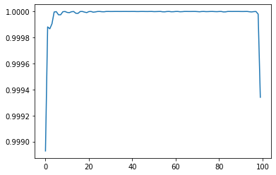
plt.plot(np.diag(mat))
plt.show()
nb_samples = 500

generated_correls = []
for i in range(nb_samples):
    noise = tf.random.normal(shape=[1, latent_dim])
    generated_image = model.sample(noise)
    correls = np.array(generated_image[0, :, :, 0])
    generated_correls.extend(list(correls[a, b]))

empirical_correls = []
for i in range(len(corrs[:min(nb_samples, len(corrs)), :, :])):
    empirical = corrs[i, :, :]
    empirical_correls.extend(list(empirical[a, b]))
len(generated_correls), len(empirical_correls)
(2475000, 2475000)
plt.hist(generated_correls, bins=100, alpha=0.5,
density=True, label='VAE correlations')
plt.hist(empirical_correls, bins=100, alpha=0.5,
density=True, label='empirical correlations')
plt.axvline(x=np.mean(generated_correls),
color='b', linestyle='dashed', linewidth=2)
plt.axvline(x=np.mean(empirical_correls),
color='r', linestyle='dashed', linewidth=2)
plt.legend()
plt.show()
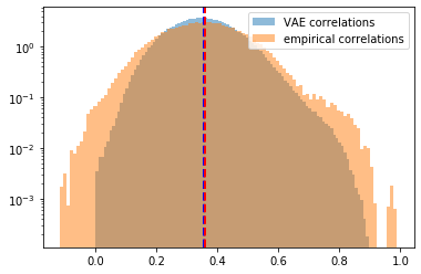
plt.hist(generated_correls, bins=100, alpha=0.5,
density=True, log=True, label='VAE correlations')
plt.hist(empirical_correls, bins=100, alpha=0.5,
density=True, log=True, label='empirical correlations')
plt.axvline(x=np.mean(generated_correls),
color='b', linestyle='dashed', linewidth=2)
plt.axvline(x=np.mean(empirical_correls),
color='r', linestyle='dashed', linewidth=2)
plt.legend()
plt.show()
from statsmodels.stats.correlation_tools import corr_nearest

nb_samples = 500

generated_corr_mats = []
for i in range(nb_samples):

    noise = tf.random.normal(shape=[1, latent_dim])
    generated_image = model.sample(noise)
    correls = np.array(generated_image[0, :, :, 0])
    # set diag to 1
    np.fill_diagonal(correls, 1)
    # symmetrize
    correls[b, a] = correls[a, b]
    # nearest corr
    nearest_correls = corr_nearest(correls)
    # set diag to 1
    np.fill_diagonal(nearest_correls, 1)
    # symmetrize
    nearest_correls[b, a] = nearest_correls[a, b]

    generated_corr_mats.append(nearest_correls)

empirical_corr_mats = []
for i in range(len(corrs[:min(nb_samples, len(corrs)), :, :])):
    empirical = corrs[i, :, :]
    empirical_corr_mats.append(empirical)
def compute_eigenvals(correls):
    eigenvalues = []
    for corr in correls:
        eigenvals, eigenvecs = np.linalg.eig(corr)
        eigenvalues.append(sorted(eigenvals, reverse=True))

    return eigenvalues

sample_mean_empirical_eigenvals = np.mean(
    compute_eigenvals(empirical_corr_mats), axis=0)
sample_mean_dcgan_eigenvals = np.mean(
    compute_eigenvals(generated_corr_mats), axis=0)
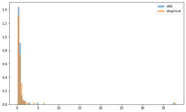
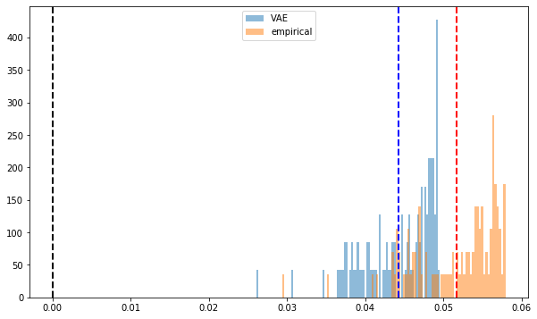
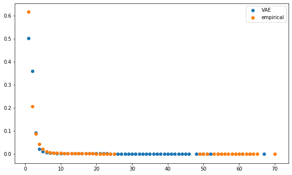
plt.figure(figsize=(10, 6))
plt.hist(sample_mean_dcgan_eigenvals, bins=n,
         density=True, alpha=0.5, label='VAE')
plt.hist(sample_mean_empirical_eigenvals, bins=n,
         density=True, alpha=0.5, label='empirical')
plt.legend()
plt.show()
def compute_pf_vec(correls):
    pf_vectors = []
    for corr in correls:
        eigenvals, eigenvecs = np.linalg.eig(corr)
        pf_vector = eigenvecs[:, np.argmax(eigenvals)]
        if len(pf_vector[pf_vector < 0]) > len(pf_vector[pf_vector > 0]):
            pf_vector = -pf_vector
        pf_vectors.append(pf_vector)

    return pf_vectors

mean_empirical_pf = np.mean(
    compute_pf_vec(empirical_corr_mats), axis=0)
mean_dcgan_pf = np.mean(
    compute_pf_vec(generated_corr_mats), axis=0)
plt.figure(figsize=(10, 6))
plt.hist(mean_dcgan_pf, bins=n, density=True,
         alpha=0.5, label='VAE')
plt.hist(mean_empirical_pf, bins=n, density=True,
         alpha=0.5, label='empirical')
plt.axvline(x=0,
            color='k', linestyle='dashed', linewidth=2)
plt.axvline(x=np.mean(mean_dcgan_pf),
            color='b', linestyle='dashed', linewidth=2)
plt.axvline(x=np.mean(mean_empirical_pf),
            color='r', linestyle='dashed', linewidth=2)
plt.legend()
plt.show()
import fastcluster
from scipy.cluster import hierarchy
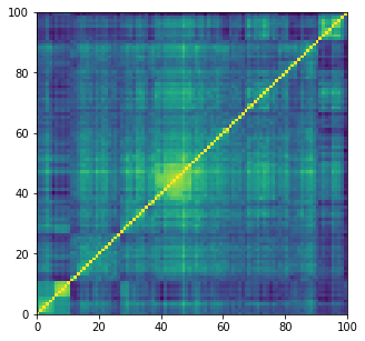
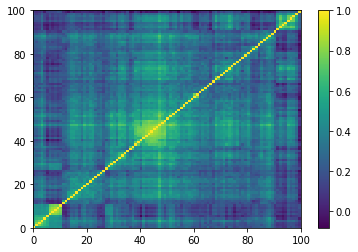
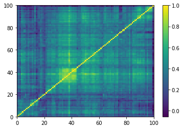
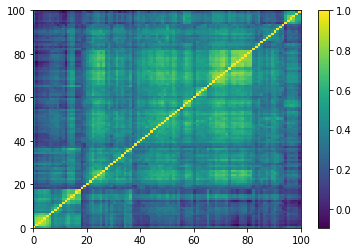
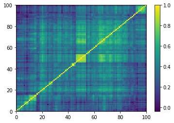
for idx, corr in enumerate(empirical_corr_mats):
dist = 1 - corr
Z = fastcluster.linkage(dist[a, b], method='ward')
permutation = hierarchy.leaves_list(
hierarchy.optimal_leaf_ordering(Z, dist[a, b]))
prows = corr[permutation, :]
ordered_corr = prows[:, permutation]
plt.pcolormesh(ordered_corr)
plt.colorbar()
plt.show()
if idx > 5:
break
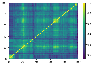
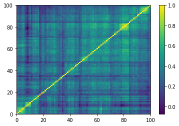
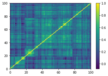
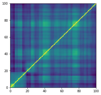
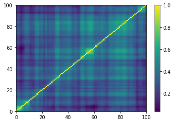
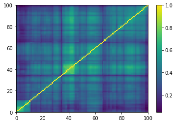
for idx, corr in enumerate(generated_corr_mats):
    dist = 1 - corr
    Z = fastcluster.linkage(dist[a, b], method='ward')
    permutation = hierarchy.leaves_list(
        hierarchy.optimal_leaf_ordering(Z, dist[a, b]))
    prows = corr[permutation, :]
    ordered_corr = prows[:, permutation]

    plt.pcolormesh(ordered_corr)
    plt.colorbar()
    plt.show()

    if idx > 5:
        break

def compute_degree_counts(correls):
    all_counts = []
    for corr in correls:
        dist = (1 - corr) / 2
        G = nx.from_numpy_matrix(dist)
        mst = nx.minimum_spanning_tree(G)

        degrees = {i: 0 for i in range(len(corr))}
        for edge in mst.edges:
            degrees[edge[0]] += 1
            degrees[edge[1]] += 1
        degrees = pd.Series(degrees).sort_values(ascending=False)
        cur_counts = degrees.value_counts()
        counts = np.zeros(len(corr))
        for i in range(len(corr)):
            if i in cur_counts:
                counts[i] = cur_counts[i]

        all_counts.append(counts / (len(corr) - 1))

    return all_counts
import networkx as nx

mean_dcgan_counts = np.mean(
    compute_degree_counts(generated_corr_mats), axis=0)
mean_dcgan_counts = (pd
                     .Series(mean_dcgan_counts)
                     .replace(0, np.nan))

mean_empirical_counts = np.mean(
    compute_degree_counts(empirical_corr_mats), axis=0)
mean_empirical_counts = (pd
                         .Series(mean_empirical_counts)
                         .replace(0, np.nan))
plt.figure(figsize=(10, 6))
plt.scatter(mean_dcgan_counts.index,
            mean_dcgan_counts,
            label='VAE')
plt.scatter(mean_empirical_counts.index,
            mean_empirical_counts,
            label='empirical')
plt.legend()
plt.show()
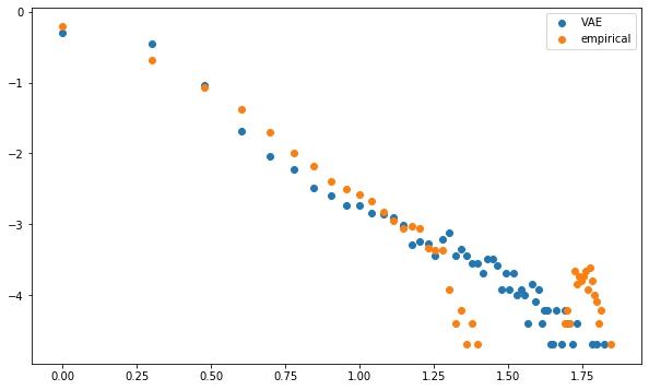
plt.figure(figsize=(10, 6))
plt.scatter(np.log10(mean_dcgan_counts.index),
            np.log10(mean_dcgan_counts),
            label='VAE')
plt.scatter(np.log10(mean_empirical_counts.index),
            np.log10(mean_empirical_counts),
            label='empirical')
plt.legend()
plt.show()