[Paper + Implementation] The Hierarchical Equal Risk Contribution Portfolio (Part I)
[Paper + Implementation] The Hierarchical Equal Risk Contribution Portfolio (Part I)
This blog post (first in a series) will discuss the paper The Hierarchical Equal Risk Contribution Portfolio by Thomas Raffinot.
I see this approach of building portfolios using hierarchical clustering a strong alternative to the approach proposed by Marcos López de Prado in his Building Diversified Portfolios That Outperform Out-of-Sample (paper, slides).
Edit: I recently became aware (thanks Marcos and Jochen for pointing it to me) that some of the ideas exposed below can be found in Jochen’s PhD thesis (2011) which you can download there: Asset Clusters and Asset Networks in Financial Risk Management and Portfolio Optimization (cf. 4.2 The Cluster Based Waterfall Approach).
In brief, some context: Empirical estimates of the correlation (or covariance) matrix are very noisy (the system is ill-defined as there are usually more variables (e.g. stocks) than observations (e.g. trading days)). Most portfolio construction methods use an inverse of the covariance matrix. Inverting the already noisy covariance matrix amplifies the noise and numerical instability. That is why sophisticated portfolio methods relying too heavily on covariance matrix estimates (or worse, its inverse) tend to underperform naive allocation methods (such as equi-weighting, aka “1/N”) out-of-sample. Some methods exist to improve the quality of the covariance (or correlation) estimate:
- Ledoit-Wolf shrinkage, Honey, I Shrunk the Sample Covariance Matrix
- Bouchaud-Potters-Bun random matrix theory, Cleaning large correlation matrices: tools from random matrix theory
- hierarchical clustering
But, usually, once the covariance matrix is “cleaned”, it is fed to a standard portfolio construction technique (e.g. mean-variance optimizer).
Marcos López de Prado, and to a greater extent Thomas Raffinot, propose to leverage the hierarchical clustering to perform the asset allocation rather than just doing the pre-processing (i.e. cleaning the covariance matrix).
The Hierarchical Risk Parity (HRP) by Marcos, and discussed already in these blogs (part 1, part 2, part 3), simply reorganizes the covariance matrix to place similar assets (in terms of linear co-movements) together, then employs an inverse-variance weighting allocation with no further use of the hierarchical structure (only the order of the assets derived from it).
Some shortcomings of the HRP methodology:
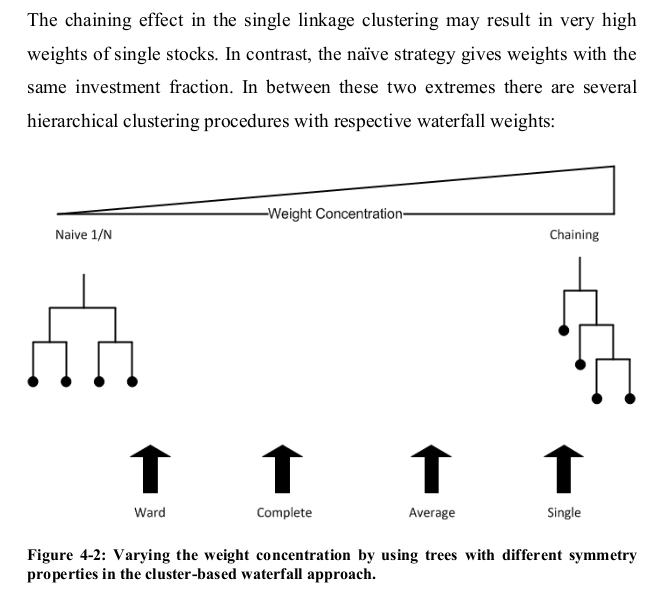
- The original HRP is based on the single-linkage (equivalent to the minimum spanning tree) algorithm, which suffers from the chaining effect: clusters are not dense enough and could span to very heterogeneous points since the algorithm merges clusters in a greedy fashion by considering only their two closest points; problem discussed in my financial clustering review
Solution: However, it is straightforward to replace the Single-Linkage by another hierarchical clustering algorithm such as Average-Linkage or Ward.
One can find in Jochen’s PhD thesis the Figure below:
- The hierarchical clustering algorithm is only used to re-order assets but the shape of the tree is not taken further into account when the bissection (asset allocation) is done (cf. picture below from the original paper). Actually, the cuts of the bissection depends only on the number of assets, which is an arbitrary quantity.
Solution: Take the shape of the dendrogram into account (cf. HERC algorithm).
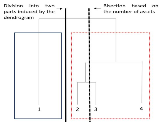
One can find in Jochen’s PhD thesis the Figure below:
- HRP doesn’t try to retrieve an appropriate number of clusters: It bisects to the leaves, i.e. until each asset is its own cluster, overfitting to the data.
In Raffinot’s words:
overfitting denotes the situation when a model targets particular observations rather than a general structure: the model explains the training data instead of finding patterns that could generalize it. In other words, attempting to make the model conform too closely to slightly inaccurate data can infect the model with substantial errors and reduce its predictive power.
Solution: Early stopping of the top-down algorithm at a prescribed level (i.e. number of clusters).
The Hierarchical Equal Risk Contribution Algorithm
-
Perform a hierarchical clustering algorithm
-
Select an appropriate number of clusters (many different methods to do it)
-
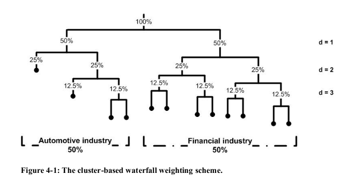
Top-Down recursive division into two parts based on the dendrogram, and following the Equal Risk Contribution allocation: $a_1 = \frac{\mathcal{RC}_1}{\mathcal{RC}_1 + \mathcal{RC}_2}$, $a_2 = 1 - a_1$, where $\mathcal{RC}_1, \mathcal{RC}_2$ are the risk contributions of the first and second clusters respectively
-
Naive Risk Parity within clusters (within a given cluster the correlation between assets should be high and relatively homogeneous)
Note that in Raffinot’s original paper there are other refinements described: For example, an extension to downside risk measures such as Conditional Value at Risk (CVaR) and Conditional Drawdown at Risk (CDaR); use of a block bootstrap to assess performance. We may explore further these refinements in follow-up studies, but, for now, we keep it simple, and use variance as our risk measure. To provide a simple example to analyze, we also use a correlation matrix instead of a covariance matrix (i.e. unit variance on the diagonal).
Below we provide a simple implementation of the algorithm that focuses on its main aspects.
%matplotlib inline

import numpy as np
import fastcluster
from scipy.cluster import hierarchy
from scipy.cluster.hierarchy import fcluster
import matplotlib.pyplot as plt
correl_mat = np.load('normal_mats/mat_5649.npy')
plt.pcolormesh(correl_mat)
plt.colorbar()
plt.show()
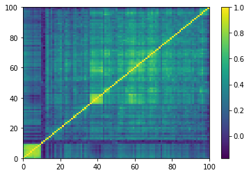
1. Perform a hierarchical clustering algorithm, and select an appropriate number of clusters
dist = 1 - correl_mat
dim = len(dist)
tri_a, tri_b = np.triu_indices(dim, k=1)
Z = fastcluster.linkage(dist[tri_a, tri_b], method='ward')
permutation = hierarchy.leaves_list(
    hierarchy.optimal_leaf_ordering(Z, dist[tri_a, tri_b]))
ordered_corr = correl_mat[permutation, :][:, permutation]

nb_clusters = 7
clustering_inds = fcluster(Z, nb_clusters, criterion='maxclust')
clusters = {i: [] for i in range(min(clustering_inds),
                                 max(clustering_inds) + 1)}
for i, v in enumerate(clustering_inds):
    clusters[v].append(i)

plt.figure(figsize=(8, 8))
plt.pcolormesh(correl_mat)
for cluster_id, cluster in clusters.items():
    xmin, xmax = min(cluster), max(cluster)
    ymin, ymax = min(cluster), max(cluster)

    plt.axvline(x=xmin,
                ymin=ymin / dim, ymax=(ymax + 1) / dim,
                color='r')
    plt.axvline(x=xmax + 1,
                ymin=ymin / dim, ymax=(ymax + 1) / dim,
                color='r')
    plt.axhline(y=ymin,
                xmin=xmin / dim, xmax=(xmax + 1) / dim,
                color='r')
    plt.axhline(y=ymax + 1,
                xmin=xmin / dim, xmax=(xmax + 1) / dim,
                color='r')
plt.show()
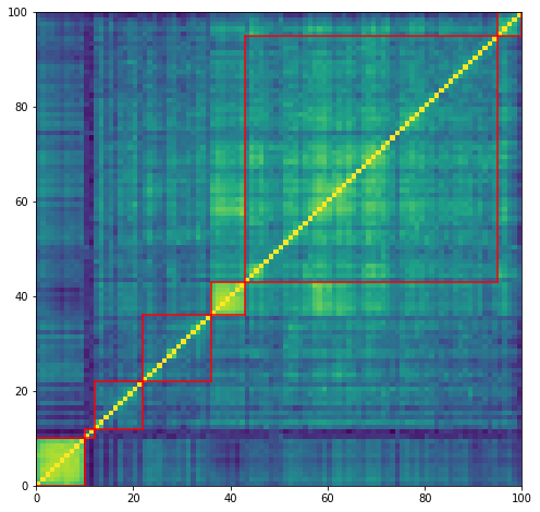
for id_cluster, cluster in clusters.items():
    print(id_cluster - 1, ':', cluster)
0 : [0, 1, 2, 3, 4, 5, 6, 7, 8, 9]
1 : [95, 96, 97, 98, 99]
2 : [36, 37, 38, 39, 40, 41, 42]
3 : [43, 44, 45, 46, 47, 48, 49, 50, 51, 52, 53, 54, 55, 56, 57, 58, 59, 60, 61, 62, 63, 64, 65, 66, 67, 68, 69, 70, 71, 72, 73, 74, 75, 76, 77, 78, 79, 80, 81, 82, 83, 84, 85, 86, 87, 88, 89, 90, 91, 92, 93, 94]
4 : [22, 23, 24, 25, 26, 27, 28, 29, 30, 31, 32, 33, 34, 35]
5 : [10, 11]
6 : [12, 13, 14, 15, 16, 17, 18, 19, 20, 21]
3. Top-Down recursive allocation, and naive risk parity within clusters
def seriation(Z, dim, cur_index):
    if cur_index < dim:
        return [cur_index]
    else:
        left = int(Z[cur_index - dim, 0])
        right = int(Z[cur_index - dim, 1])
        return seriation(Z, dim, left) + seriation(Z, dim, right)

def intersection(lst1, lst2):
    return list(set(lst1) & set(lst2))
def compute_allocation(covar, clusters):
    nb_clusters = len(clusters)
    assets_weights = np.array([1.] * len(covar))
    clusters_weights = np.array([1.] * nb_clusters)
    clusters_var = np.array([0.] * nb_clusters)

    for id_cluster, cluster in clusters.items():
        cluster_covar = covar[cluster, :][:, cluster]
        inv_diag = 1 / np.diag(cluster_covar)
        assets_weights[cluster] = inv_diag / np.sum(inv_diag)

    for id_cluster, cluster in clusters.items():
        weights = assets_weights[cluster]
        clusters_var[id_cluster - 1] = np.dot(
            weights, np.dot(covar[cluster, :][:, cluster], weights))

    for merge in range(nb_clusters - 1):
        print('id merge:', merge)
        left = int(Z[dim - 2 - merge, 0])
        right = int(Z[dim - 2 - merge, 1])
        left_cluster = seriation(Z, dim, left)
        right_cluster = seriation(Z, dim, right)

        print(len(left_cluster),
              len(right_cluster))

        ids_left_cluster = []
        ids_right_cluster = []
        for id_cluster, cluster in clusters.items():
            if sorted(intersection(left_cluster, cluster)) == sorted(cluster):
                ids_left_cluster.append(id_cluster)
            if sorted(intersection(right_cluster, cluster)) == sorted(cluster):
                ids_right_cluster.append(id_cluster)


        ids_left_cluster = np.array(ids_left_cluster) - 1
        ids_right_cluster = np.array(ids_right_cluster) - 1
        print(ids_left_cluster)
        print(ids_right_cluster)
        print()

        alpha = 0
        left_cluster_var = np.sum(clusters_var[ids_left_cluster])
        right_cluster_var = np.sum(clusters_var[ids_right_cluster])
        alpha = left_cluster_var / (left_cluster_var + right_cluster_var)

        clusters_weights[ids_left_cluster] = clusters_weights[
            ids_left_cluster] * alpha
        clusters_weights[ids_right_cluster] = clusters_weights[
            ids_right_cluster] * (1 - alpha)

    for id_cluster, cluster in clusters.items():
        assets_weights[cluster] = assets_weights[cluster] * clusters_weights[
            id_cluster - 1]

    return assets_weights
And, finally, we get the weights of the assets (summing to 1):
weights = compute_allocation(correl_mat, clusters)
We display below the successive merging of clusters: 6 merges for 7 clusters. First, the algorithm merges clusters with ids 2 and 3 of size 7 and 52 respectively, then clusters with ids 5 and 6 of size 2 and 10 respectively, then cluster of id 1 and size 5 with the cluster composed of sub-clusters 2 and 3 having now a size 7 + 52 = 59 giving birth to a cluster with ids 1, 2, 3 of size 5 + 59 = 64, etc. until the last merge which gathers cluster of id 0 and size 10 with the big cluster of size 90 composed by the sub-clusters 1, 2, 3, 4, 5, 6.
id merge: 0
10 90
[0]
[1 2 3 4 5 6]

id merge: 1
64 26
[1 2 3]
[4 5 6]

id merge: 2
14 12
[4]
[5 6]

id merge: 3
5 59
[1]
[2 3]

id merge: 4
2 10
[5]
[6]

id merge: 5
7 52
[2]
[3]
Below, we illustrate the distribution of weights on the different clusters:
plt.figure(figsize=(8, 8))
plt.pcolormesh(correl_mat)
for cluster_id, cluster in clusters.items():
    xmin, xmax = min(cluster), max(cluster)
    ymin, ymax = min(cluster), max(cluster)

    plt.axvline(x=xmin,
                ymin=ymin / dim, ymax=(ymax+1) / dim,
                color='r')
    plt.axvline(x=xmax+1,
                ymin=ymin / dim, ymax=(ymax+1) / dim,
                color='r')
    plt.axhline(y=ymin,
                xmin=xmin / dim, xmax=(xmax+1) / dim,
                color='r')
    plt.axhline(y=ymax+1,
                xmin=xmin / dim, xmax=(xmax+1) / dim,
                color='r')
plt.show()
plt.figure(figsize=(8, 2))
plt.plot(weights)
plt.xlim([0, 100])
plt.show()

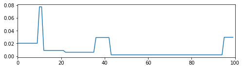
Conclusion: In this blog, we provide a simple implementation of the HERC. We will experiment more with this method, and its extensions, in follow-up studies to get an intuitive feel of its results. Also, we would like to compare HERC to similar methods such as HRP, Hierarchical “1/N” (a particular case of HERC), and standard portfolio allocation techniques. To do so, and aiming at a scientifically valid result, we will use statistical techniques such as block bootstrapping time series of returns, or even applying these methods on samples generated from a GAN or a VAE (in the spirit of CorrGAN).
Jochen concludes on his seminal presentation of these hierarchical allocation methods:
- The waterfall rule is static and there is not much room for weight adjustments (e.g. investment constraints)
- […]
- Turnover rates can be higher than in benchmark models
- Dendrogram heights have not yet been incorporated
To the best of my knowledge, these problems have not yet been solved so far.