[Book] Commented summary of Machine Learning for Asset Managers by Marcos Lopez de Prado
[Book] Commented summary of Machine Learning for Asset Managers by Marcos Lopez de Prado
Did a quick reading of Marcos’ new book over the week-end.
Overall, a (very) good read.
Interesting, not because it contains new mathematical developments or ideas (most of the clustering related content is between 10 to 20 years old; same for the random matrix theory (RMT) part, which is already applied in many hedge funds and other sophisticated asset managers), but because all these existing ideas and methods (prevalent in the industry or in (some part of, e.g. econophysics rather than finance) academia) are, maybe for the first time, exposed clearly and linearly throughout the book. You may find RMT experts, clustering experts, optimizers in chief, and various frameworks to deal with multiple testing biases, but rarely all this knowledge is brought together in one place with a consistent presentation and set of notations. Marcos has achieved this, by clearly exposing all these elements (if not the most recent sophistications).
The below contains excerpts that I found interesting or worth flagging: Essentially, high level comments rather than technical parts.
Important part of my graduate research and PhD thesis (and occasional blogging) is aligned with the book: the importance of using synthetic data, various uses of (hierarchical) clustering (risk, portfolio construction, relative value), developing alternative ways of measuring dependence (aka non-linear correlations). Based on my research experience, I add some personal comments to a few excerpts, when I disagree or just to bring an alternative point of view.
You can buy it on Amazon: Machine Learning for Asset Managers (Elements in Quantitative Finance)
Chapter 1 Introduction
Only a few years ago, it was rare to find ML applications outside short-term price prediction, trade execution, and setting of credit ratings.
Firms that resist this revolution will likely share Kodak’s fate.
Machine Learning for Asset Managers is concerned with answering a different challenge: how can we use ML to build better financial theories?
A historical simulation of an investment strategy’s performance (backtest) is not a theory; it is a (likely unrealistic) simulation of a past that never happened (you did not deploy that strategy years ago; that is why you are backtesting it!).
Contrary to popular belief, backtesting is not a research tool. Backtests can never prove that a strategy is a true positive, and they may only provide evidence that a strategy is a false positive. Never develop a strategy solely through backtests.
The most insightful use of ML in finance is for discovering theories. You may use ML successfully for making financial forecasts; however, that is not necessarily the best scientific use of this technology (particularly if your goal is to develop high-capacity investment strategies).
The black box view of ML is a misconception. It is fueled by popular industrial applications of ML, where the search for better predictions outweighs the need for theoretical understanding.
Another example of test set overfitting occurs when a researcher backtests a strategy and she tweaks it until the output achieves a target performance. That backtest–tweak–backtest cycle is a futile exercise that will inevitably end with an overfit strategy (a false positive).
In other words, a poorly performing backtest is an opportunity to fix the research process, not an opportunity to fix a particular investment strategy.
Many research questions involve the notion of similarity or distance. For example, we may be interested in understanding how closely related two variables are. Denoised covariance matrices can be very useful for deriving distance metrics from linear relationships. Modeling nonlinear relationships requires more advanced concepts. Section 3 provides an information-theoretic framework for extracting complex signals from noisy data. In particular, it allows us to define distance metrics with minimal assumptions regarding the underlying variables that characterize the metric space. These distance metrics can be thought of as a nonlinear generalization of the notion of correlation.
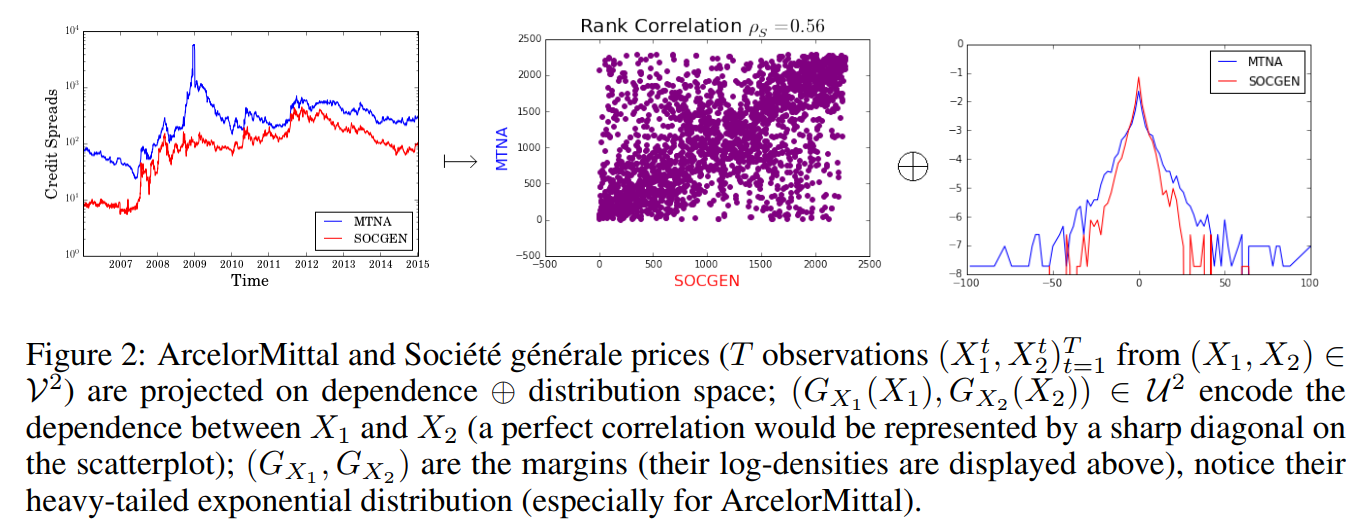
Essentially a big part of my PhD thesis Chapter 5 Distances between financial time series: non-linear measures of dependence (copula-based), coupled with a distance between the marginal behaviour. In short, distance between two variables = distance in correlation between them + distance between their distribution.
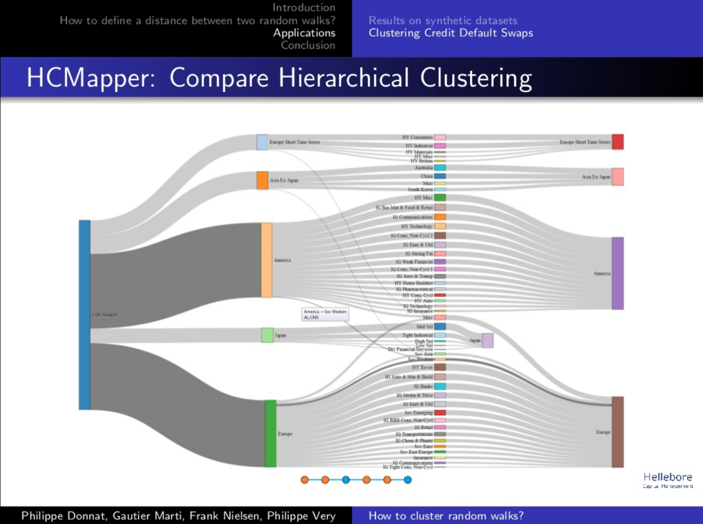
Cf. also this paper, co-authored with Philippe Very, and Philippe Donnat, using both credit default swap spreads and synthetic time series to illustrate the point.
One of the applications of distance matrices is to study whether some variables are more closely related among themselves than to the rest, hence forming clusters. Clustering has a wide range of applications across finance, like in asset class taxonomy, portfolio construction, dimensionality reduction, or modeling networks of agents.
Cf. my review of two decades of correlations, hierarchies, networks and clustering in financial markets.
ML models can be interpreted through a number of procedures, such as PDP, ICE, ALE, Friedman’s H-stat, MDI, MDA, global surrogate, LIME, and Shapley values, among others.
ML is a black box reveals how some people have chosen to apply ML, and it is not a universal truth.
Conclusions drawn from millions of Monte Carlo simulations teach us something about the general mathematical properties of a particular approach. The anecdotal evidence derived from a handful of historical simulations is no match to evaluating a wide range of scenarios.
Other financial ML applications, like sentiment analysis, deep hedging, credit ratings, execution, and private commercial data sets, enjoy an abundance of data.
Finally, in some settings, researchers can conduct randomized controlled experiments, where they can generate their own data and establish precise cause–effect mechanisms. For example, we may reword a news article and compare ML’s sentiment extraction with a human’s conclusion, controlling for various changes.
Because the signal-to-noise ratio is so low in finance, data alone are not good enough for relying on black box predictions. That does not mean that ML cannot be used in finance. It means that we must use ML differently, hence the notion of financial ML as a distinct subject of study. Financial ML is not the mere application of standard ML to financial data sets. Financial ML comprises ML techniques specially designed to tackle the specific challenges faced by financial researchers, just as econometrics is not merely the application of standard statistical techniques to economic data sets.
The goal of financial ML ought to be to assist researchers in the discovery of new economic theories. The theories so discovered, and not the ML algorithms, will produce forecasts. This is no different than the way scientists utilize ML across all fields of research.
Perhaps the most popular application of ML in asset management is price prediction. But there are plenty of equally important applications, like hedging, portfolio construction, detection of outliers and structural breaks, credit ratings, sentiment analysis, market making, bet sizing, securities taxonomy, and many others. These are real-life applications that transcend the hype often associated with expectations of price prediction.
For example, factor investing firms use ML to redefine value. A few years ago, price-to-earnings ratios may have provided a good ranking for value, but that is not the case nowadays. Today, the notion of value is much more nuanced. Modern asset managers use ML to identify the traits of value, and how those traits interact with momentum, quality, size, etc.
High-frequency trading firms have utilized ML for years to analyze real-time exchange feeds, in search for footprints left by informed traders. They can utilize this information to make short-term price predictions or to make decisions on the aggressiveness or passiveness in order execution. Credit rating agencies are also strong adopters of ML, as these algorithms have demonstrated their ability to replicate the ratings generated by credit analysts. Outlier detection is another important application, since financial models can be very sensitive to the presence of even a small number of outliers. ML models can help improve investment performance by finding the proper size of a position, leaving the buy-or-sell decision to traditional or fundamental models.
I am particularly excited about real-time prediction of macroeconomic statistics, following the example of MIT’s Billion Prices Project.
The computational power and functional flexibility of ML ensures that it will always find a pattern in the data, even if that pattern is a fluke rather than the result of a persistent phenomenon.
I have never heard a scientist say “Forget about theory, I have this oracle that can answer anything, so let’s all stop thinking, and let’s just believe blindly whatever comes out.”
Imagine if physicists had to produce theories in a universe where the fundamental laws of nature are in a constant flux; where publications have an impact on the very phenomenon under study; where experimentation is virtually impossible; where data are costly, the signal is dim, and the system under study is incredibly complex
One of the greatest misunderstandings I perceive from reading the press is the notion that ML’s main (if not only) objective is price prediction.
Having an edge at price prediction is just one necessary, however entirely insufficient, condition to be successful in today’s highly competitive market. Other areas that are equally important are data processing, portfolio construction, risk management, monitoring for structural breaks, bet sizing, and detection of false investment strategies, just to cite a few.
Chapter 2 Denoising and Detoning
Not much Machine Learning, but standard application of Random Matrix Theory to the estimation of correlation (covariance) matrices.
This chapter essentially describes an approach that Bouchaud and his crew from the CFM have pioneered and refined for the past 20 years. The latest iteration of this body of work is summarized in Joel Bun’s Cleaning large correlation matrices: Tools from Random Matrix Theory.
See Lewandowski et al. (2009) for alternative ways of building a random covariance matrix.
Cf. The Onion Method.
Methods presented in the Chapter:
Constant Residual Eigenvalue Method
Targeted Shrinkage
and following the denoising:
Detoning
Without loss of generality, the variances are drawn from a uniform distribution bounded between 5% and 20%
Would be more realistic to sample from a multimodal distribution.
We can further reduce the condition number by reducing the highest eigenvalue. This makes mathematical sense, and also intuitive sense. Removing the market components present in the correlation matrix reinforces the more subtle signals hiding under the market “tone.” For example, if we are trying to cluster a correlation matrix of stock returns, detoning that matrix will likely help amplify the signals associated with other exposures, such as sector, industry, or size.
Chapter 3 Distance Metrics
My topic of “expertise” (alongside clustering algorithms for financial time series, cf. PhD defense slides which I studied and researched with Frank Nielsen, expert in computational information theory/geometry.
Estimation of mutual information can be quite brittle. It relies on a good binning of an, in general, unbounded support, which is hard to achieve. Instead, it can be better to consider copulas (even to estimate mutual information, as mutual information between two variables is the negative entropy of their copula density, a distribution defined on $[0, 1] \times [0, 1]$, cf. computation below).
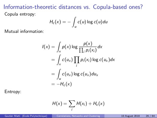
That is mutual information is yet another projection from the copula to a scalar supposed to measure a certain aspect of the dependence between two variables. Others can be studied and used…
A paper that summarizes my understanding of 2d non-linear dependence, Exploring and measuring non-linear correlations: Copulas, Lightspeed Transportation and Clustering, and some related slides.
But before we can do that, we need to address a technical problem: correlation is not a metric, because it does not satisfy nonnegativity and triangle inequality conditions. Metrics are important because they induce an intuitive topology on a set. Without that intuitive topology, comparing non-metric measurements of codependence can lead to rather incoherent outcomes. For instance, the difference between correlations (0.9,1.0) is the same as (0.1,0.2), even though the former involves a greater difference in terms of codependence.
This is not due to the metric property, but rather the properties of the metric itself.
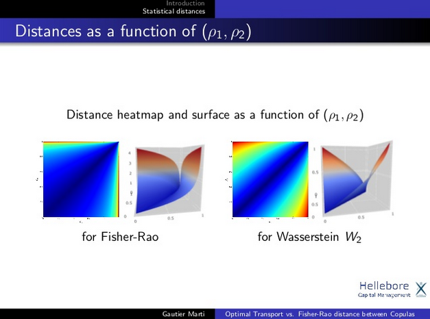
Cf. the first part of this blog to see the curvature implied by a Riemannian distance between two correlations.
Cf. also the two slides below:
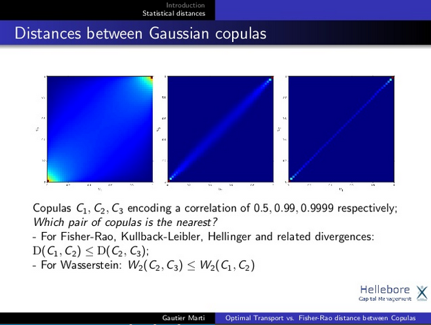 It depends on the metric chosen, not on the fact it is a metric or not. For some applications the curvature implied by information theory metrics are more suitable, for others a flatter geometry such as the onde induced by the Optimal Transport / Euclidean geometry are more relevant.
 For some applications the curvature implied by information theory metrics are more suitable, for others a flatter geometry such as the one induced by the Optimal Transport / Euclidean geometry are more relevant.
We may compute the correlation between any two real variables, however that correlation is typically meaningless unless the two variables follow a bivariate Normal distribution. To overcome these caveats, we need to introduce a few information-theoretic concepts.
Not the only approach available. Cf. copula theory.
3.9 Discretization
In an empirical setting, this binning/discretization process is source of instability, especially with variables having an unbounded (or widely varying) range. That’s a reason why optimal transport which can be defined on empirical measures can be a good alternative to the f-divergences (information theoretic pseudo-metrics) which are defined for absolutely continuous measures, and thus require a Kernel Density Estimation (KDE) pre-processing (another potential source for introducing noise and instability).
As we can see from these equations, results may be biased by our choice of BX and BY [the number of bins].
In the context of unsupervised learning, variation of information is useful for comparing outcomes from a partitional (non-hierarchical) clustering algorithm.
3.11 Experimental Results
A bit naive, but rather pedagogical like the rest of this chapter. Dependence measures are well studied and understood in the statistical literature. I do believe that many (most?) asset managers are familiar with the non-linear, information theoretic, copula (and others) alternative dependence measures. Are they using them though? Why? Why not? Only a third order improvement? I can guess that reporting to non-quants (compliance, management, and clients), and other, unrelated to market, risks can prevent their main street adoption. In short, business constraints could outweight the benefits.
From a personal perspective, I stopped (more accurately, dramatically slowed down) my research in the exploitation of non-linear dependence, as I could feel it is both too niche at the moment, and is not the major driver of pnl… Still keeping an eye open on the research though.
For nonlinear cases, we have argued that the normalized variation of information is a more appropriate distance metric.
Not the only one.
It allows us to answer questions regarding the unique information contributed by a random variable, without having to make functional assumptions.
But there are other assumptions, and pitfalls in the estimation: from a scatter plot to absolutely continuous measures.
Given that many ML algorithms do not impose a functional form on the data, it makes sense to use them in conjunction with entropy-based features.
Chapter 4 Optimal Clustering
Clustering problems appear naturally in finance, at every step of the investment process. For instance, analysts may look for historical analogues to current events, a task that involves developing a numerical taxonomy of events.
Portfolio managers often cluster securities with respect to a variety of features, to derive relative values among peers.
Risk managers are keen to avoid the concentration of risks in securities that share common traits.
Traders wish to understand flows affecting a set of securities, to determine whether a rally or sell-off is idiosyncratic to a particular security, or affects a category shared by a multiplicity of securities.
This section focuses on the problem of finding the optimal number and composition of clusters.
Vaste programme.
Clusters are modeled on two dimensions, features and observations. An example is biclustering (also known as coclustering). For instance, they can help identify similarities in subsets of instruments and time periods simultaneously.
The clustering of correlation matrices is peculiar in the sense that the features match the observations: we try to group observations where the observations themselves are the features (hence the symmetry of X). Matrix X appears to be a distance matrix, but it is not. It is still an observations matrix, on which distances can be evaluated.
A sort of distance of distances approach. I happen to do it a few times, provides usually more optically salient clusters. Not totally sure though about the practice of using a similarity (or dissimilairty matrix) as the observations to compute yet another distance matrix on top, and apply the clustering on it. Why not. In my usual toolbox, I directly apply clustering on the correlation matrix (transformed into a dissimilarity matrix by a simple pointwise transformation). Might be worth a bit more investigation to compare the two approaches, and their impact on downstream tasks.
In short, the book applies the clustering on an observation matrix. If you have a correlation matrix at hand, the book suggests you to cast it into an observation matrix first.
4.4.2 Base Clustering
At this stage, we assume that we have a matrix that expresses our observations in a metric space.
4.5 Experimental Results
Both the algorithm to find the optimal number of clusters, and the Monte Carlo experiment using a block-diagonal model are a bit naive. The algorithm recovers the blocks injected in the model, but this is an extremely simplified model of what we can usually observe in a real data empirical setting. I have also been guilty of using such simplified models times and times over (e.g. in there or there). That is why I have started my project on CorrGAN, a GAN that can learn realistic hierarchical (correlation) matrices structure, and generate new ones at will for more realistic Monte Carlo simulations.
Is MSCI’s GICS classification system an example of hierarchical or partitioning clustering? Using the appropriate algorithm on a correlation matrix, try to replicate the MSCI classification. To compare the clustering output with MSCI’s, use the clustering distance introduced in Section 3.
That’s quite a poor way of comparing the two classifications. Since the trading universes are usually not so large (at most a few thousands of assets, more often in the hundreds), I find it better to visualize and explore interactively the differences with some d3.js visualization.
Chapter 5 Financial Labels
Researchers need to ponder very carefully how they define labels, because labels determine the task that the algorithm is going to learn.
For example, we may train an algorithm to predict the sign of today’s return for stock XYZ, or whether that stock’s next 5% move will be positive (a run that spans a variable number of days). The features needed to solve both tasks can be very different, as the first label involves a point forecast whereas the second label relates to a path-dependent event. For example, the sign of a stock’s daily return may be unpredictable, while a stock’s probability of rallying (unconditional on the time frame) may be assessable.
That some features failed to predict one type of label for a particular stock does not mean that they will fail to predict all types of labels for that same stock.
Four labeling strategies:
5.2 Fixed-Horizon Method
5.3 Triple-Barrier Method
5.4 Trend-Scanning Method
5.5 Meta-labeling
The fixed-horizon method, although implemented in most financial studies, suffers from multiple limitations. Among these limitations, we listed that the distribution of fixed-horizon labels may not be stationary, that these labels dismiss path information, and that it would be more practical to predict the side of the next absolute return that exceeds a given threshold.
Chapter 6 Feature Importance Analysis
In this section, we demonstrate that ML provides intuitive and effective tools for researchers who work on the development of theories. Our exposition runs counter to the popular myth that supervised ML models are black-boxes. According to that view, supervised ML algorithms find predictive patterns, however researchers have no understanding of those findings. In other words, the algorithm has learned something, not the researcher. This criticism is unwarranted.
6.2 p-Values
The misuse of p-values is so widespread that the American Statistical Association has discouraged their application going forward as a measure of statistical significance (Wasserstein et al. 2019). This casts a doubt over decades of empirical research in Finance. In order to search for alternatives to the p-value, first we must understand its pitfalls.
In summary, p-values require that we make many assumptions (caveat #1) in order to produce a noisy estimate (caveat #2) of a probability that we do not really need (caveat #3), and that may not be generalizable out-of-sample (caveat #4).
6.3 Feature Importance
This section suggests solutions based on feature importance techniques.
A better approach, which does not require a change of basis, is to cluster similar features and apply the feature importance analysis at the cluster level. By construction, clusters are mutually dissimilar, hence taming the substitution effects. Because the analysis is done on a partition of the features, without a change of basis, results are usually intuitive.
The MDI and MDA methods assess the importance of features robustly and without making strong assumptions about the distribution and structure of the data.
Furthermore, unlike p-values, clustered MDI and clustered MDA estimates effectively control for substitution effects. But perhaps the most salient advantage of MDI and MDA is that, unlike classical significance analyses, these ML techniques evaluate the importance of a feature irrespective of any particular specification.
Once the researcher knows the variables involved in a phenomenon, she can focus her attention on finding the mechanism or specification that binds them together.
Chapter 7 Portfolio Construction
There are three popular approaches to reducing the instability in optimal portfolios. First, some authors attempted to regularize the solution, by injecting additional information regarding the mean or variance in the form of priors (Black and Litterman 1992). Second, other authors suggested reducing the solution’s feasibility region by incorporating additional constraints (Clarke et al. 2002). Third, other authors proposed improving the numerical stability of the covariance matrix’s inverse (Ledoit and Wolf 2004).
López de Prado (2016) introduced an ML-based asset allocation method called hierarchical risk parity (HRP). HRP outperforms Markowitz and the naïve allocation in out-of-sample Monte Carlo experiments. The purpose of HRP was not to deliver an optimal allocation, but merely to demonstrate the potential of ML approaches. In fact, HRP outperforms Markowitz out-ofsample even though HRP is by construction suboptimal in-sample.
I re-implemented the HRP method some time ago and experimented with it in several blogs: HRP part I, HRP part II, HRP part III.
Note also that there was around, since 2011, a competitive method by Papenbrock based on similar insights, which was rediscovered and improved more recently by Raffinot. This competitive approach is described and implemented in this blog.
We can contain that instability by optimizing the dominant clusters separately, hence preventing that the instability spreads throughout the entire portfolio.
The remainder of this section is dedicated to introducing a new ML-based method, named nested clustered optimization (NCO), which tackles the source of Markowitz’s curse.
Note to self: re-implement and experiment with it.
Code Snippet 7.7 creates a random vector of means and a random covariance matrix that represent a stylized version of a fifty securities portfolio, grouped in ten blocks with intracluster correlations of 0.5.
Throughout this book, the correlation (covariance) models are a bit naive. I shall re-implement all the experiments using CorrGAN, and the soon-to-be-released conditional CorrGAN.
Markowitz’s portfolio optimization framework is mathematically correct, however its practical application suffers from numerical problems. In particular, financial covariance matrices exhibit high condition numbers due to noise and signal. The inverse of those covariance matrices magnifies estimation errors, which leads to unstable solutions: changing a few rows in the observations matrix may produce entirely different allocations. Even if the allocations estimator is unbiased, the variance associated with these unstable solutions inexorably leads to large transaction costs than can erase much of the profitability of these strategies.
In finance, where clusters of securities exhibit greater correlation among themselves than to the rest of the investment universe, eigenvalue functions are not horizontal, which in turn is the cause for high condition numbers. Signal is the cause of this type of covariance instability, not noise.
Like many other ML algorithms, NCO is flexible and modular. For example, when the correlation matrix exhibits a strongly hierarchical structure, with clusters within clusters, we can apply the NCO algorithm within each cluster and subcluster, mimicking the matrix’s tree-like structure.
This is the the idea of the The Hierarchical Equal Risk Contribution Portfolio by Thomas Raffinot: Distribute the weights in a hierarchical fashion (following the dendrogram structure), and stop at some prescribed level (a relevant number of clusters) since going deeper would likely yield to overfit random correlation coefficients.
The goal is to contain the numerical instability at each level of the tree, so that the instability within a subcluster does not extend to its parent cluster or the rest of the correlation matrix.
2 Repeat Section 7.7, where this time you generate covariance matrices without a cluster structure, using the function getRndCov listed in Section 2. Do you reach a qualitatively different conclusion? Why?
I did that for HRP (HRP part II vs. HRP part III). Basically, if your algorithm is designed to leverage a hierarchical structure, and there is none, no particular advantage.
4 Repeat Section 7.7 for a covariance matrix of size ten and for a covariance matrix of size one hundred. How do NCO’s results compare to Markowitz’s as a function of the problem’s size?
The bigger, the better…
Chapter 8 Testing Set Overfitting
It is easy for a researcher to overfit a backtest, by conducting multiple historical simulations, and selecting the best performing strategy (Bailey et al. 2014).
To make matters worse, SBuMT [selection bias under multiple testing] is compounded at many asset managers, as a consequence of sequential SBuMT at two levels: (1) each researcher runs millions of simulations, and presents the best (overfit) ones to her boss; (2) the company further selects a few backtests among the (already overfit) backtests submitted by the researchers.
Financial analysts do not typically assess the performance of a strategy in terms of precision and recall. The most common measure of strategy performance is the Sharpe ratio. In what follows, we will develop a framework for assessing the probability that a strategy is false. The inputs are the Sharpe ratio estimate, as well as metadata captured during the discovery process.
New developments from the original paper presenting the deflated Sharpe ratio, which I played with and implemented in this blog How to detect false strategies? The Deflated Sharpe Ratio some time ago.
The content of this chapter would deserve I experiment more with it to have a better intuitive understanding of the numerical behaviour of all these formulas. Possibly more blogs to come.
Appendix A: Testing on Synthetic Data
Contains a brief summary of most of the techniques available to the research to generate synthetic data, from the old classical statistics ones (such as Jackknife and Bootstrap) to mentions of the most recent computational ones (such as variational autoencoders and generative adversarial networks), which I have been exploring for the past year (with varying success).