Measuring non-linear dependence with Optimal Transport
Measuring non-linear dependence with Optimal Transport
In this short blog, I re-implement a dependence measure I introduced some time ago in my PhD research. This dependence measure is based on Optimal Transport (OT). At the time, I had to (with much help from Sebastien Andler) implement all the primitives around (e.g. OT distance, Wasserstein barycenter, Sinkhorn distances), and it was rather slow…
In the meantime, a specialized Python library has appeared and matured POT: Python Optimal Transport. This gives me a good occasion to re-implement bits of Exploring and measuring non-linear correlations: Copulas, Lightspeed Transportation and Clustering to get familiar with it.
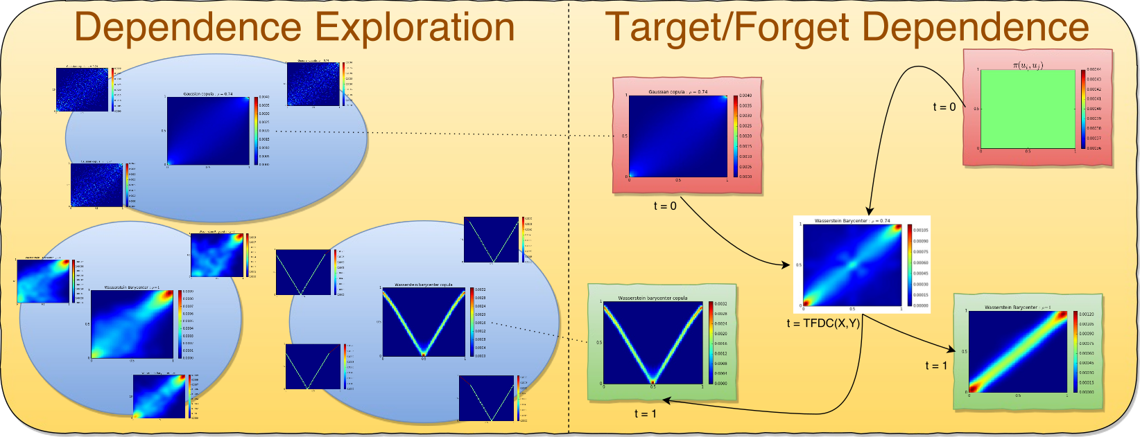
The basic idea of the optimal copula transport dependence measure is rather simple. It relies on leveraging:
-
copulas, which are distributions encoding fully the dependence between random variables,
-
a geometrical point of view: Where does the empirical copula stand in the space of copulas? In particular, how far is it from reference copulas such as the Fréchet–Hoeffding copula bounds (copulas associated to comonotone, countermonotone, independent random variables)?
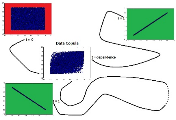
Dependence is measured as the relative distance from independence to the nearest target-dependence: comonotonicity or countermonotonicity.
Optimal Transport provides distances which are well suited for empirical distributions with free support (no need of binning or other density estimation techniques which may add up noise in the process); cf. this presentation comparing OT to classic divergences.
%matplotlib inline

import numpy as np
from scipy.stats import (
    spearmanr, pearsonr, kendalltau,
    rankdata)
import ot
import matplotlib.pyplot as plt
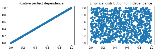
Let’s define two reference copulas: positive dependence, and independence
nb_obs = 1000

target = np.array([[i / nb_obs, i / nb_obs]
                   for i in range(nb_obs)])
forget = np.array([[u, v]
                   for u, v in zip(np.random.uniform(size=nb_obs),
                                   np.random.uniform(size=nb_obs))])
plt.figure(figsize=(10, 6))
plt.subplot(2, 2, 1)
plt.scatter(target[:, 0],
            target[:, 1])
plt.title('Positive perfect dependence')

plt.subplot(2, 2, 2)
plt.scatter(forget[:, 0],
            forget[:, 1])
plt.title('Empirical distribution for independence')
plt.show()
Definition of the optimal copula transport dependence measure (a particular case)
def compute_copula_ot_dependence(empirical, target, forget):
    # uniform distribution on samples
    t_measure, f_measure, e_measure = (
        np.ones((nb_obs,)) / nb_obs,
        np.ones((nb_obs,)) / nb_obs,
        np.ones((nb_obs,)) / nb_obs)
    # compute the ground distance matrix between locations
    gdist_e2t = ot.dist(empirical, target)
    gdist_e2f = ot.dist(empirical, forget)
    # compute the optimal transport matrix
    e2t_ot = ot.emd(t_measure, e_measure, gdist_e2t)
    e2f_ot = ot.emd(f_measure, e_measure, gdist_e2f)
    # compute the optimal transport distance:
    # <optimal transport matrix, ground distance matrix>_F
    e2t_dist = np.trace(np.dot(np.transpose(e2t_ot), gdist_e2t))
    e2f_dist = np.trace(np.dot(np.transpose(e2f_ot), gdist_e2f))
    # compute the copula ot dependence measure
    return 1 - e2t_dist / (e2f_dist + e2t_dist)
Random variables useful for the experiment
Note that the variance of an uniform random variable on $[0,1]$ is 1/12.
# random variables: Z ~ U[0,1], eps_X, eps_Y ~ N(0, 1/12)
Z = np.random.uniform(size=nb_obs)
eps_X = np.random.normal(scale=np.sqrt(1/12), size=nb_obs)
eps_Y = np.random.normal(scale=np.sqrt(1/12), size=nb_obs)
np.std(Z), np.std(eps_X), np.std(eps_Y)
(0.28543945948413835, 0.2795327636484723, 0.2768787531952918)
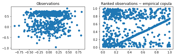
Let’s define two random variables $X, Y$ such that $X = Z \mathbf{1}_{Z < a} + \epsilon_X \mathbf{1}_{Z > a}, Y = Z \mathbf{1}_{Z < a + 1/4} + \epsilon_Y \mathbf{1}_{Z > a + 1/4}$, where $Z \sim \mathcal{U}[0,1], \epsilon_X, \epsilon_Y \sim \mathcal{N}(0, 1/12)$, and $a \in [0, 1]$.
# example of the dependence relation on one instance
threshold = 0.5

X = [z if z < threshold else ex
         for z, ex in zip(Z, eps_X)]
Y = [z if z < threshold + 1 / 4 else ey
     for z, ey in zip(Z, eps_Y)]

Xunif = rankdata(X) / len(X)
Yunif = rankdata(Y) / len(Y)

plt.figure(figsize=(10, 6))
plt.subplot(2, 2, 1)
plt.scatter(X, Y)
plt.title('Observations')
plt.subplot(2, 2, 2)
plt.scatter(Xunif, Yunif)
plt.title('Ranked observations ~ empirical copula')
plt.show()
Experiment
Let’s vary $a \in [0,1]$. We should measure more dependence between $X$ and $Y$ with $a$ increasing.
pearsons = []
spearmans = []
kendalls = []
copula_ots = []

plt.figure(figsize=(10, 10))
for idx, threshold in enumerate(np.linspace(0, 1, 100)):

    X = [z if z < threshold else ex
         for z, ex in zip(Z, eps_X)]
    Y = [z if z < threshold + 1 / 4 else ey
         for z, ey in zip(Z, eps_Y)]

    Xunif = rankdata(X) / len(X)
    Yunif = rankdata(Y) / len(Y)

    empirical = np.array(
        [[x, y] for x, y in zip(Xunif, Yunif)])


    rho = pearsonr(X, Y)[0]
    rhoS = spearmanr(X, Y)[0]
    tau = kendalltau(X, Y)[0]
    copula_ot = compute_copula_ot_dependence(
        empirical, target, forget)

    pearsons.append(rho)
    spearmans.append(rhoS)
    kendalls.append(tau)
    copula_ots.append(copula_ot)
    plt.subplot(10, 10, idx + 1)
    plt.scatter(rankdata(X), rankdata(Y))
    plt.axis('off')
plt.show()

plt.figure(figsize=(15, 6))
plt.plot(np.linspace(0, 1, 100),
         pearsons, label='pearson')
plt.plot(np.linspace(0, 1, 100),
         spearmans, label='spearman')
plt.plot(np.linspace(0, 1, 100),
         kendalls, label='kendall')
plt.plot(np.linspace(0, 1, 100),
         copula_ots, label='copula ot')
plt.legend()
plt.title('Comparison of Copula OT dependence measure to standard correlations',
          fontsize=20)
plt.ylabel("Correlation measure", fontsize=16)
plt.xlabel("Threshold $a$ in $X = Z\mathbf{1}_{Z < a} + \epsilon_X\mathbf{1}_{Z > a}, Y = Z\mathbf{1}_{Z < a + 1/4} + \epsilon_Y\mathbf{1}_{Z > a + 1/4}$",
           fontsize=16)
plt.show()
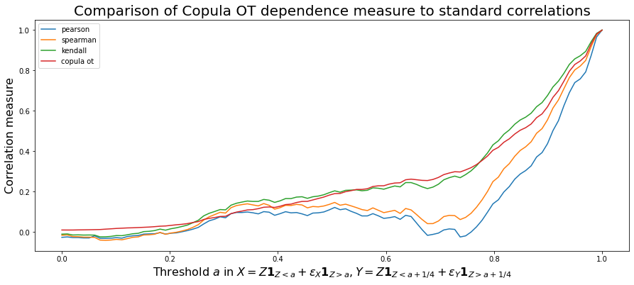
Conclusion: On this simple example, the optimal copula transport dependence measure is increasing with $a$ (the expected behaviour). Kendall $\tau$ too behaves well. This is not the case for Spearman (linear on ranks) and Pearson (linear) correlations.
With this geometric view,
-
it is rather easy to extend this novel dependence measure to alternative use cases (e.g. by changing the reference copulas).
-
It can also allow to look for specific patterns in the dependence structure (generalization of conditional correlation): Typically, one would try to answer “What is the correlation between these two stocks knowing that the VIX is above 40?” (e.g. estimate $\rho_{XY|Z>z}$); With this optimal copula transport tool, one can look for answers to, for example,
a. “Which pairs of assets are both positively and negatively correlated?”
b. “Which assets occur extreme variations while those of others are relatively small, and conversely?”
c. “Which pairs of assets are positively correlated for small variations but uncorrelated otherwise?”
To learn more about optimal transport and copula theory, I would recommend these two books: