Mutual Information Is Copula Entropy
Mutual Information Is Copula Entropy
Linear correlation, when applied to asset returns and other financial variables, has many well documented flaws: It only captures linear dependence between the variables, and its estimation is brittle to outliers (these outliers can be tails from a taily distribution, not necessarily data collection/processing outliers).
For all its defaults, linear correlation is rather easy to estimate, manipulate, and work with mathematically. A few of the reasons why it is still widespread.
For the past couple of decades, many alternative dependence measures have been developped and studied. One notable (besides the optimal copula transport one, ahah joking, or … am I?) is the Mutual Information.
Mutual Information, grounded in information theory and mathematical entropy, is supposed to capture all sorts of non-linear dependence, and hence is an interesting candidate for many application domains (e.g. science, engineering, quantitative finance).
In this blog post, we will show however that the shortcomings of its standard estimation defeats its whole purpose: estimation of mutual information is easy and accurate on Gaussians, but breaks as soon as applied on observations that follow a more taily distribution…
However, a little known connection to copula theory helps design a better and more robust estimator of Mutual Information.
In this rather obscure paper, authors make the connection between mutual information and copulas: Mutual Information Is Copula Entropy.
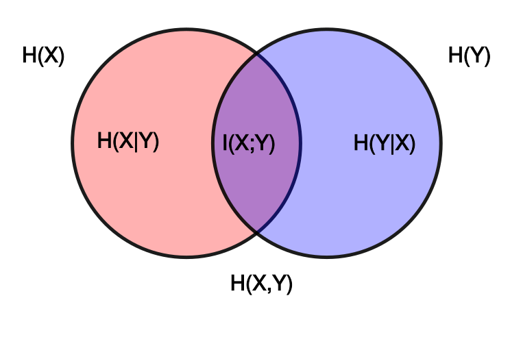
The main observation: Mutual information is a measure of dependence between two variables $X$ and $Y$: Why should we care about the margins at all? Standard estimators follow closely the well-known relation $I(X; Y) = H(X) - H(X|Y) = H(Y) - H(Y|X) = H(X) + H(Y) - H(X, Y)$, and thus need to estimate the entropy of the marginals $H(X)$ and $H(Y)$.
Continuous marginals (think the distribution of returns of each stock) have a potentially unbounded support making it hard to bin properly. The discretization process to estimate the density, which is needed to compute the entropy, may introduce biases in the mutual information estimate due to a rather difficult and arbitrary binning of the support.
Using their copula $C(X, Y)$, which is super easy to estimate (Deheuvels has shown that a normalized ranking of the observations is a very good estimator of the underlying copula), allows to bypass the estimation of the margins. One can either estimate the copula $C$, and apply the standard mutual information estimator on it (the copula has compact support in $[0, 1]^2$, its margins are uniform), or compute $(-1) \times$ the copula entropy.
TL;DR Mutual information can be tricky to estimate. In most cases, it is poorly done, and may be worse than using a simple linear correlation. A simple yet powerful connection to copula theory, namely $MI = - H(C)$, allows to obtain a robust estimator which is also easy and fast to compute.
%matplotlib inline

import numpy as np
from scipy.stats import (
    entropy, rankdata, pearsonr, spearmanr)
from scipy.special import beta, digamma
from sklearn.metrics import mutual_info_score
import matplotlib.pyplot as plt


def estimate_mutual_information(X, Y, nb_bins=100):
    joint = np.histogram2d(X, Y, nb_bins)[0]
    return mutual_info_score(None, None, contingency=joint)
The easiest possible statistical setup: Experiment with a bivariate Gaussian, i.e. a Gaussian copula with Gaussian margins
Let’s generate observations following a bivariate Gaussian.
rho = 0.5
nb_observations = 10000
mean = [0, 0]
var_X = 120
var_Y = 0.1
cov = [[var_X, rho * np.sqrt(var_X) * np.sqrt(var_Y)],
       [rho * np.sqrt(var_X) * np.sqrt(var_Y), var_Y]]

observations = np.random.multivariate_normal(mean=mean,
                                             cov=cov,
                                             size=nb_observations)
We know an analytical expression for the mutual information of two variables following a bivariate Gaussian distribution of correlation $\rho$: $I(X; Y) = -\frac{1}{2} \log(1 - \rho^2)$.
analytical_mutual_information = - 0.5 * np.log(1 - rho**2)

analytical_mutual_information
0.14384103622589045
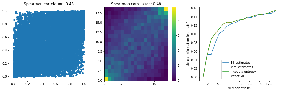
Conveniently, there are formulas to help find an optimal binning for the discretization:
nb_bins_opt = int(
    round((1 / np.sqrt(2)) * np.sqrt(1 + np.sqrt(
        1 + 24 * len(observations) / (1 - rho**2)))))

nb_bins_opt
17
X_unif = rankdata(observations[:, 0]) / len(observations)
Y_unif = rankdata(observations[:, 1]) / len(observations)

copula_density = np.histogram2d(X_unif, Y_unif,
                                bins=nb_bins_opt, density=True)[0]


estimates = []
c_estimates = []
max_bins = int(nb_bins_opt * 1.2)
for b in range(1, max_bins):
    estimates.append(estimate_mutual_information(observations[:, 0],
                                                 observations[:, 1],
                                                 nb_bins=b))
    c_estimates.append(estimate_mutual_information(
        rankdata(observations[:, 0]) / len(observations),
        rankdata(observations[:, 1]) / len(observations),
        nb_bins=b))

ce = []
for b in range(1, max_bins):
    copula_density = np.histogram2d(X_unif, Y_unif, bins=b, density=True)[0]
    copula_freq = np.histogram2d(X_unif, Y_unif, bins=b, density=False)[0]
    bin_area = (copula_freq / copula_density / len(observations))[0, 0]
    c = copula_density.ravel() + 1e-9
    ce.append(sum(c * np.log(c) * bin_area))


plt.figure(figsize=(16, 4.5))
plt.subplot(1, 3, 1)
plt.scatter(X_unif, Y_unif)
plt.title('Spearman correlation: {}'.format(
    round(spearmanr(X_unif, Y_unif)[0], 2)))

plt.subplot(1, 3, 2)
plt.pcolormesh(copula_density)
plt.title('Spearman correlation: {}'.format(
    round(spearmanr(X_unif, Y_unif)[0], 2)))
plt.colorbar()

plt.subplot(1, 3, 3)
plt.plot(range(1, max_bins), estimates, label='MI estimates')
plt.plot(range(1, max_bins), c_estimates, label='c MI estimates')
plt.plot(range(1, max_bins), ce, label='- copula entropy')
plt.axhline(analytical_mutual_information, c='k', label='exact MI')
plt.axvline(nb_bins_opt, c='purple')
plt.xlabel('Number of bins')
plt.ylabel('Mutual information (estimate)')
plt.legend()
plt.show()
copula_density = np.histogram2d(X_unif, Y_unif,
                                bins=nb_bins_opt, density=True)[0]
copula_freq = np.histogram2d(X_unif, Y_unif,
                             bins=nb_bins_opt, density=False)[0]
bin_area = (copula_freq / copula_density / len(observations))[0, 0]
c = copula_density.ravel() + 1e-9

mi_hat = estimate_mutual_information(observations[:, 0],
                                     observations[:, 1],
                                     nb_bins=nb_bins_opt)

print('Copula entropy estimator: {}\nStandard esimator: {}\nanalytical (true) value: {}'.format(
    round(sum(c * np.log(c) * bin_area), 4),
    round(mi_hat, 4),
    round(analytical_mutual_information, 4)))
Copula entropy estimator: 0.1481
Standard esimator: 0.1482
analytical (true) value: 0.1438
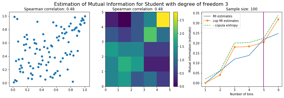
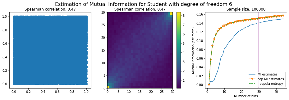
Experiment with a bivariate Student-t distribution, i.e. a Student-t copula with Student-t margins
A harder statistical setting where mutual information should shine.
Multivariate Student-t is a distribution which essentially depends on a mean and a covariance matrix, like the Gaussian, but also on a parameter called the degree of freedom which parameterizes how heavy are the tails. When the degree of freedom parameter tends to infinity, the multivariate Student-t tends to a Gaussian distribution. The lower the parameter, the heavier the tails.
Student-t exhibits both tail-dependence (two stocks can crash or rally big at the same time; a 0 probability event according to the Gaussian copula) and tail-values (a stock can move by much more than what would be expected from a Normal distribution of returns).
NB For the family of elliptical copulas, to whom Student-t belongs, Spearman correlation (linear correlation on ranks) or Kendall $\tau$ (concordance measure of ranks) are particularly well suited, and I think preferable to mutual information.
def multivariate_student(mean, cov, dof, size):
    d = len(cov)
    g = np.tile(np.random.gamma(dof / 2., 2. / dof, size), (d, 1)).T
    Z = np.random.multivariate_normal(np.zeros(d), cov, size)
    return mean + Z / np.sqrt(g)
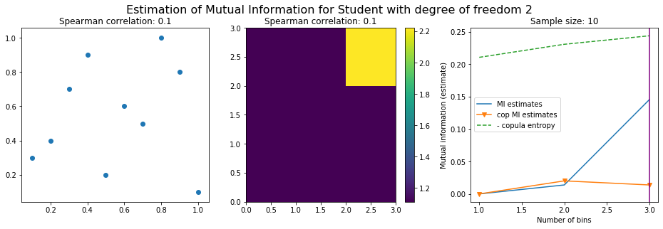
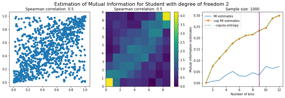
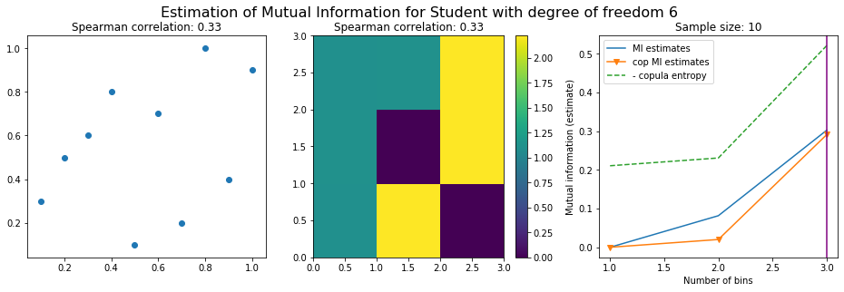
For this numerical experiment, we will consider 3 possible values for the degree of freedom (dof): 2 (variance undefined), 3 (heavy tails), 6 (relatively less heavy tailed, more Gaussian-ish).
For each dof parameter, we will consider a regular binning of b bins, looping through a wide range of reasonable values.
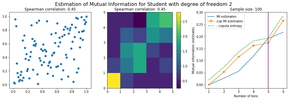
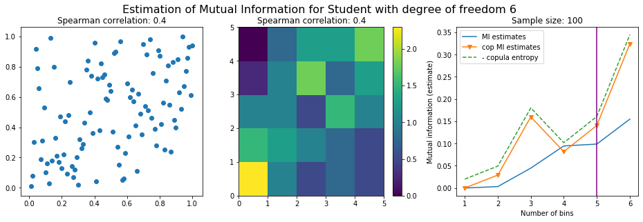
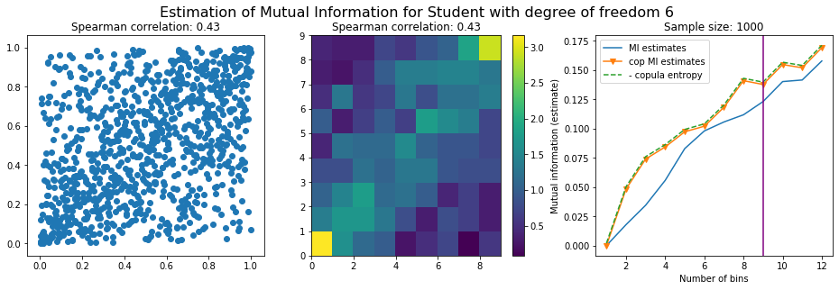
We plot the mutual information estimates for all these combinations, and for three estimators:
a. standard Mutual Information estimator (blue line)
b. standard Mutual Information estimator applied to the copula and its uniform margins (orange line)
c. estimation of (-1) * entropy of the copula (dashed green line)
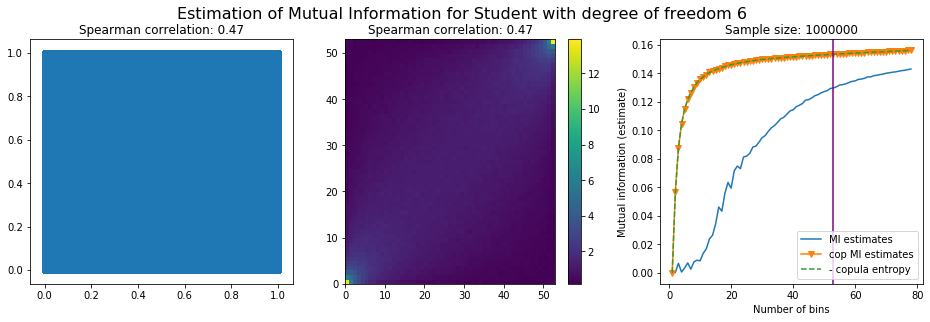
The experiment below essentially shows that the mutual information estimates are:
-
strongly dependent on the number of bins,
-
the standard estimator is brittle and uneffective with heavy tails,
-
the copula entropy estimator is more robust,
-
both estimators need a relatively large sample size,
-
the copula entropy estimator is more data efficient.
rho = 0.5
mean = [0, 0]
var_X = 120
var_Y = 0.1
cov = [[var_X, rho * np.sqrt(var_X) * np.sqrt(var_Y)],
       [rho * np.sqrt(var_X) * np.sqrt(var_Y), var_Y]]

for dof in [2, 3, 6]:

    for size in [10**i for i in range(1, 7)]:
        observations = multivariate_student(mean, cov, dof, size)
        nb_bins_opt = int(
        round((1 / np.sqrt(2)) * np.sqrt(1 + np.sqrt(
            1 + 24 * len(observations) / (1 - rho**2)))))

        X_unif = rankdata(observations[:, 0]) / len(observations)
        Y_unif = rankdata(observations[:, 1]) / len(observations)

        estimates = []
        c_estimates = []
        max_bins = int(nb_bins_opt * 1.5)
        for b in range(1, max_bins):
            estimates.append(estimate_mutual_information(observations[:, 0],
                                                         observations[:, 1],
                                                         nb_bins=b))
            c_estimates.append(estimate_mutual_information(
                rankdata(observations[:, 0]) / len(observations),
                rankdata(observations[:, 1]) / len(observations),
                nb_bins=b))

        ce = []
        for b in range(1, max_bins):
            copula_density = np.histogram2d(X_unif, Y_unif,
                                            bins=b, density=True)[0]
            copula_freq = np.histogram2d(X_unif, Y_unif,
                                         bins=b, density=False)[0]
            bin_area = (copula_freq / copula_density / len(observations))[0, 0]
            c = copula_density.ravel() + 1e-9
            ce.append(sum(c * np.log(c) * bin_area))


        plt.figure(figsize=(16, 4.5))

        plt.subplot(1, 3, 1)
        plt.scatter(X_unif, Y_unif)
        plt.title('Spearman correlation: {}'.format(
            round(spearmanr(X_unif, Y_unif)[0], 2)))

        copula_density = np.histogram2d(X_unif, Y_unif,
                                        bins=nb_bins_opt, density=True)[0]

        plt.subplot(1, 3, 2)
        plt.pcolormesh(copula_density)
        plt.title('Spearman correlation: {}'.format(
            round(spearmanr(X_unif, Y_unif)[0], 2)))
        plt.colorbar()

        plt.subplot(1, 3, 3)
        plt.plot(range(1, max_bins), estimates, label='MI estimates')
        plt.plot(range(1, max_bins), c_estimates, '-v',
            label='cop MI estimates')
        plt.plot(range(1, max_bins), ce, '--', label='- copula entropy')
        plt.axvline(nb_bins_opt, c='purple')
        plt.xlabel('Number of bins')
        plt.ylabel('Mutual information (estimate)')
        plt.legend()
        plt.title('Sample size: {}'.format(size))
        plt.suptitle(
            'Estimation of Mutual Information for Student with degree of freedom {}\n\n'
            .format(dof), fontsize=16)
        plt.show()


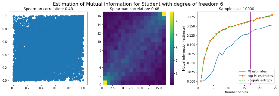
Conclusion: We have illustrated in this blog that standard mutual information estimators can behave poorly, even on large sample size. They are meant to capture non-linear dependence, but are actually struggling in (at least some of) these cases. On the contrary, the little known connection between copula entropy and mutual information gives a much better estimator of this quantity thanks to the good properties of the copula (compact support, uniform margins, easy and efficient estimator available).
For those who really need to use mutual information, I would recommend to test both estimators and compare results before acting blindly on them. Otherwise, I would recommend using optimal copula transport ;)
To go further, books I recommend reading:
Edit: Following Lionel Yelibi’s remark on how this would compare to Kraskov et al. estimator described in Estimating Mutual Information, I would like to precise a few things after reading carefully the article.
-
Copula-based estimators and Kraskov’s estimator are not really competitors: Kraskov et al. main idea is to use k-nearest neighbours instead of binning. Copula-based estimator main idea is to discard the marginals (entropy of $\mathcal{U}[0,1] = \ln(1) = 0)$. This $k$-NN technique, instead of the binning part, can be applied to the copula-based estimators described above as well.
-
Kraskov and co-authors were close to find the connection to copulas, but did not follow the idea to its end. One can see that in the paragraph below excerpt from the paper:
Often, MI is estimated after rank ordering the data, i.e. after replacing the coordinate $x_i$ by the rank of the $i$-th point when sorted by magnitude. This is equivalent to applying a monotonic transformation $x \rightarrow x’$, $y \rightarrow y’$ to each coordinate which leads to a strictly uniform empirical density, $\mu_x’(x’) = \mu_y’(x’) = (1/N) \sum_{i=1}^N \delta(x’ − i)$. For $N \rightarrow \infty$ and $k \gg 1$ this clearly leaves the MI estimate invariant. But it is not obvious that it leaves invariant also the estimates for finite $k$, since the transformation is not smooth at the smallest length scale. We found numerically that rank ordering gives correct estimates also for small $k$, if the distance degeneracies implied by it are broken by adding low amplitude noise as discussed above. In particular, both estimators still gave zero MI for independent pairs. Although rank ordering can reduce statistical errors, we did not apply it in the following tests, and we did not study in detail the properties of the resulting estimators.
- For future research: Would the copula-based mutual information estimators be improved significantly by using Kraskov k-nearest neighbours idea?