Sampling from Empirical Copulas of Stocks
Sampling from Empirical Copulas of Stocks
This short blog is a follow-up of Wasserstein Barycenters of Stocks Empirical Copulas, with much overlap.
What’s new here: We sample $n$ observations $(u, v) \in [0, 1]^2$ according to the empirical copula distribution.
So, this is as much a small tutorial on how to sample from empirical cumulative distribution function (CDF) histograms as preparing a baseline for CopulaGAN, which hopefully will extend to higher dimensions than the histogram-based method.
For convenience, the code is repeated below:
%matplotlib inline

import pandas as pd
import numpy as np
from scipy.stats import rankdata
from scipy.cluster import hierarchy
import ot
import fastcluster
import matplotlib.pyplot as plt
df = pd.read_csv('data/SP500_HistoTimeSeries.csv')
df = df.set_index('Date')
df.index = pd.to_datetime(df.index)
df = df.sort_index()
df = df.fillna(method='ffill', limit=5)
del df['SPX Index']
returns = df.pct_change()

recent_returns = returns.iloc[-252 * 4:]

for col in recent_returns:
    try:
        if (len(recent_returns[col].dropna()) <
            len(recent_returns[col])):
            del recent_returns[col]
        if col not in industry_tickers:
            del recent_returns[col]
    except:
        pass
recent_returns.shape
(1008, 478)
corr_returns = recent_returns.corr()
# sorting by hierarchical clustering
dist = 1 - corr_returns.values
dim = len(dist)
tri_a, tri_b = np.triu_indices(dim, k=1)
Z = fastcluster.linkage(dist[tri_a, tri_b], method='ward')
permutation = hierarchy.leaves_list(
hierarchy.optimal_leaf_ordering(Z, dist[tri_a, tri_b]))
HC_tickers = recent_returns.columns[permutation]
HC_corr = corr_returns.values[permutation, :][:, permutation]
nb_clusters = 9
dist = 1 - HC_corr
dim = len(dist)
tri_a, tri_b = np.triu_indices(dim, k=1)
Z = fastcluster.linkage(dist[tri_a, tri_b], method='ward')
clustering_inds = hierarchy.fcluster(Z, nb_clusters,
criterion='maxclust')
clusters = {i: [] for i in range(min(clustering_inds),
max(clustering_inds) + 1)}
for i, v in enumerate(clustering_inds):
clusters[v].append(i)
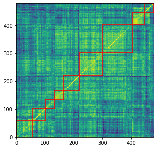
plt.figure(figsize=(5, 5))
plt.pcolormesh(HC_corr)
for cluster_id, cluster in clusters.items():
xmin, xmax = min(cluster), max(cluster)
ymin, ymax = min(cluster), max(cluster)
plt.axvline(x=xmin,
ymin=ymin / dim, ymax=(ymax + 1) / dim,
color='r')
plt.axvline(x=xmax + 1,
ymin=ymin / dim, ymax=(ymax + 1) / dim,
color='r')
plt.axhline(y=ymin,
xmin=xmin / dim, xmax=(xmax + 1) / dim,
color='r')
plt.axhline(y=ymax + 1,
xmin=xmin / dim, xmax=(xmax + 1) / dim,
color='r')
plt.show()
Now, we depart from the previous blog by computing the barycenters with more supporting ‘diracs’ than the original empirical measures. This increased ‘density’ will help for the subsequent sampling (higher resolution of the histogram).
mean_copula_large_support = {}
for i, cluster in enumerate(clusters):
    tickers = [HC_tickers[ind] for ind in clusters[cluster]]

    measures_locations = []
    measures_weights = []
    for id1, ticker1 in enumerate(tickers):
        r1 = recent_returns[ticker1]
        for id2, ticker2 in enumerate(tickers):
            if id2 > id1:
                    r2 = recent_returns[ticker2]
                    ranks = (pd
                             .concat([pd.Series(r1),
                                      pd.Series(r2)],
                                     axis=1, keys=['U', 'V'])
                             .dropna()
                             .rank(method='first'))
                    unifs = ranks / len(ranks)

                    measures_locations.append(unifs.values)
                    measures_weights.append(
                        np.array([1 /  len(unifs)
                                  for i in range(len(unifs))]))

    # the support for the mean will have M times more 'diracs'
    # than the input measures
    M = 2
    size = len(measures_locations[0]) * M
    X_init = np.vstack((np.random.uniform(size=size),
                        np.random.uniform(size=size))).T
    k = size
    b = np.ones((k,)) / k

    random_ids = np.random.randint(
        0, len(measures_locations),
        size=min(200, len(measures_locations)))
    locations = [measures_locations[idx]
                 for idx in random_ids]
    weights = [measures_weights[idx]
               for idx in random_ids]

    X = ot.lp.free_support_barycenter(
        locations, weights, X_init, b,
        numItermax=10000)

    mean_copula_large_support[i] = X
plt.figure(figsize=(17, 34))
for i in range(len(mean_copula_large_support)):
    plt.subplot(6, 3, i + 1)
    plt.scatter(mean_copula_large_support[i][:, 0],
                mean_copula_large_support[i][:, 1])

for i in range(len(mean_copula_large_support)):
    plt.subplot(6, 3, i + 9 + 1)
    hist, x_bins, y_bins = np.histogram2d(
        mean_copula_large_support[i][:, 0],
        mean_copula_large_support[i][:, 1],
        bins=30)
    plt.pcolormesh(hist)
plt.show()
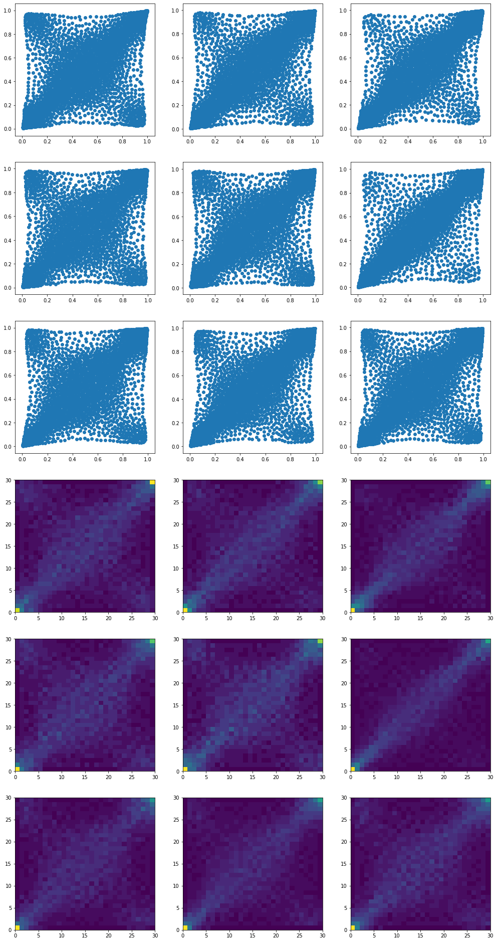
Each one of these 9 barycenters is the result of an optimization problem whose solution is supported by twice as much ‘diracs’ than the inputs.
They describe the same distributions as in the previous blog, but with a higher resolution.
Finally, we draw samples from these empirical distributions:
def sample_from_cdf(margins, size=500, nb_bins=100):
    hist, x_bins, y_bins = np.histogram2d(
        margins[:, 0], margins[:, 1], bins=(nb_bins, nb_bins))
    x_bin_midpoints = x_bins[:-1] + np.diff(x_bins) / 2
    y_bin_midpoints = y_bins[:-1] + np.diff(y_bins) / 2

    cdf = np.cumsum(hist.ravel())
    cdf = cdf / cdf[-1]

    values = np.random.uniform(size=size)
    value_bins = np.searchsorted(cdf, values)

    x_idx, y_idx = np.unravel_index(
        value_bins, (len(x_bin_midpoints), len(y_bin_midpoints)))

    random_from_cdf = np.column_stack(
        (x_bin_midpoints[x_idx], y_bin_midpoints[y_idx]))
    new_x, new_y = random_from_cdf.T

    return new_x, new_y
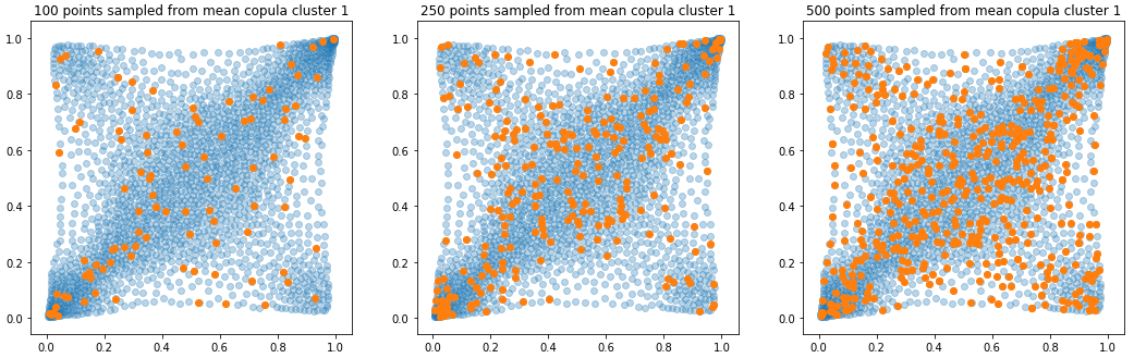
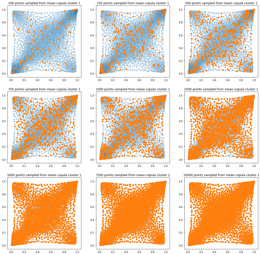
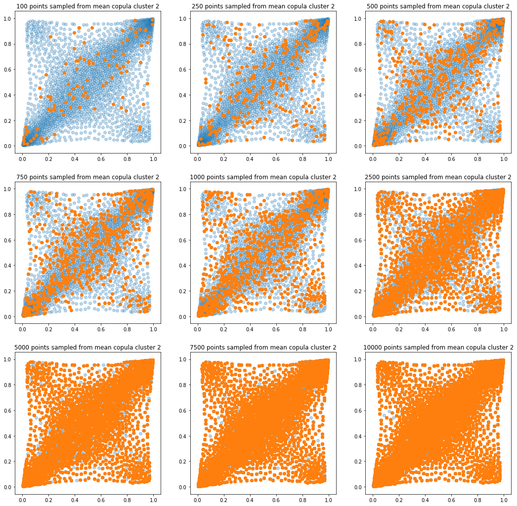
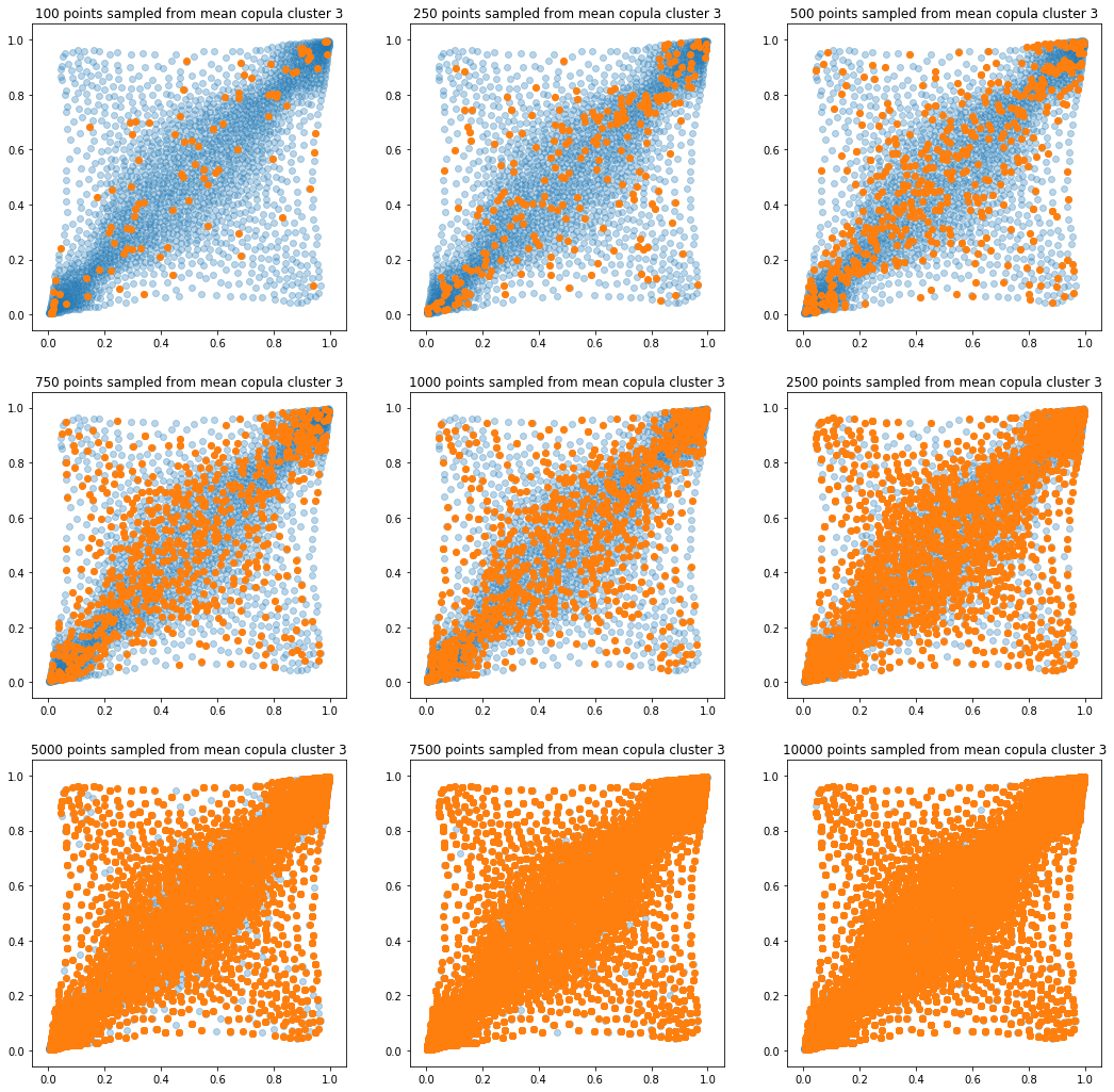
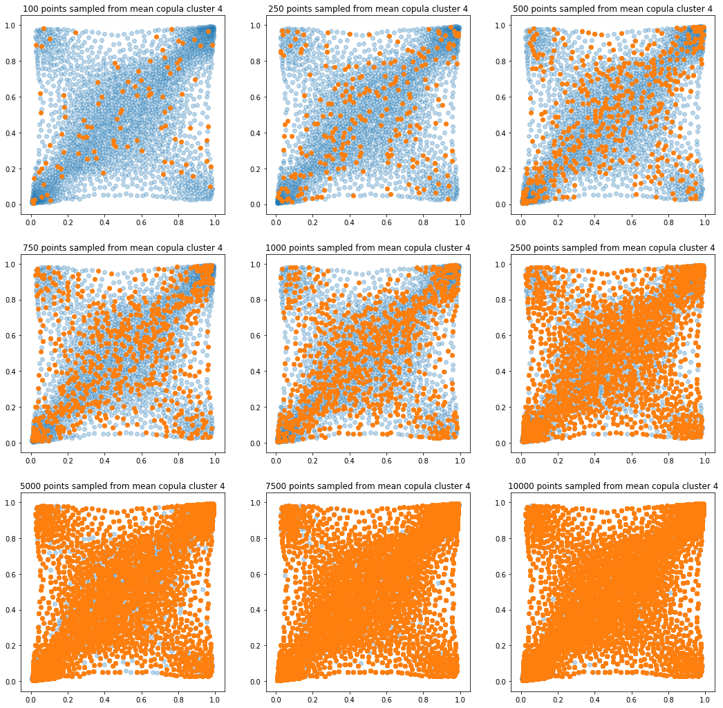
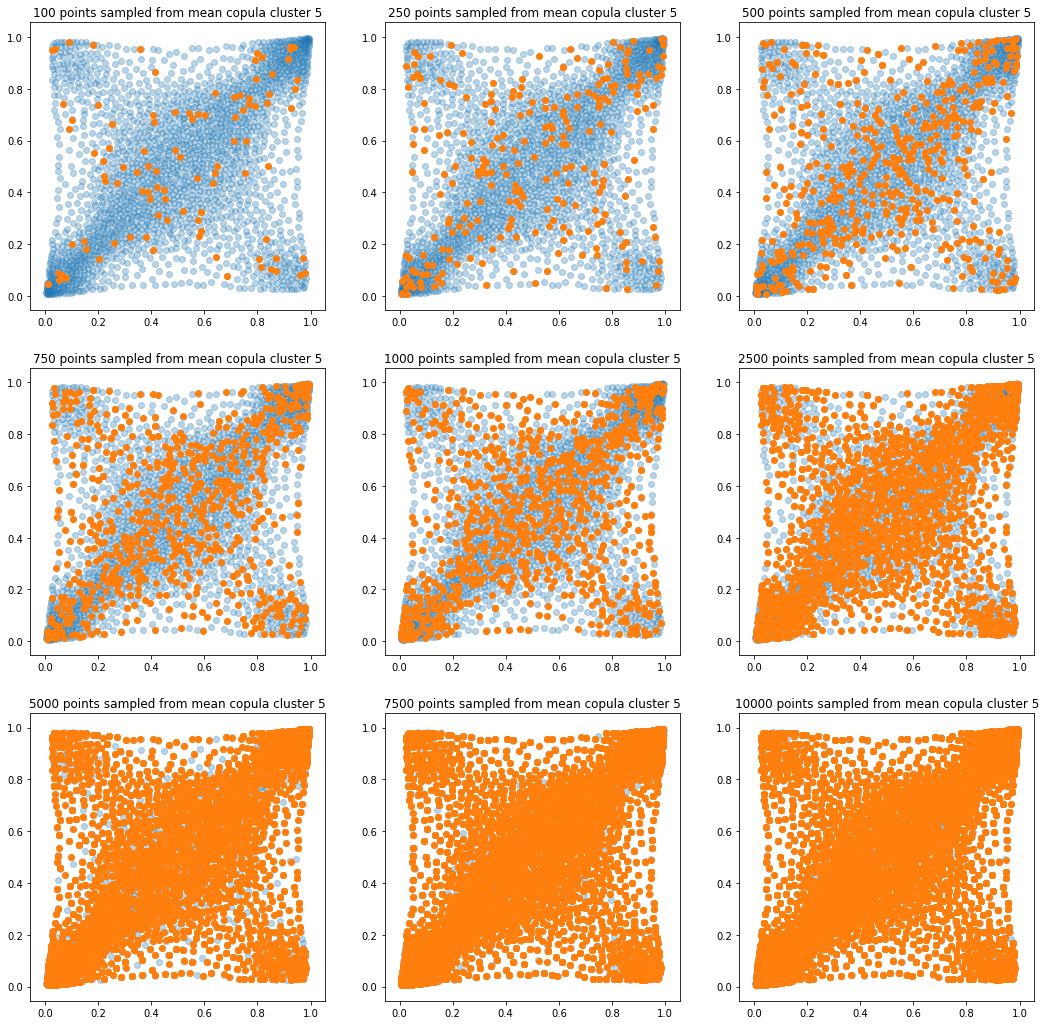
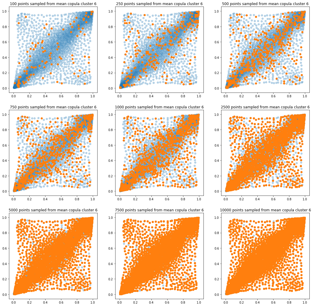
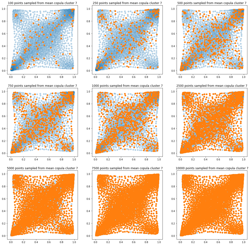
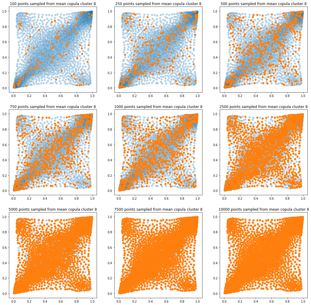
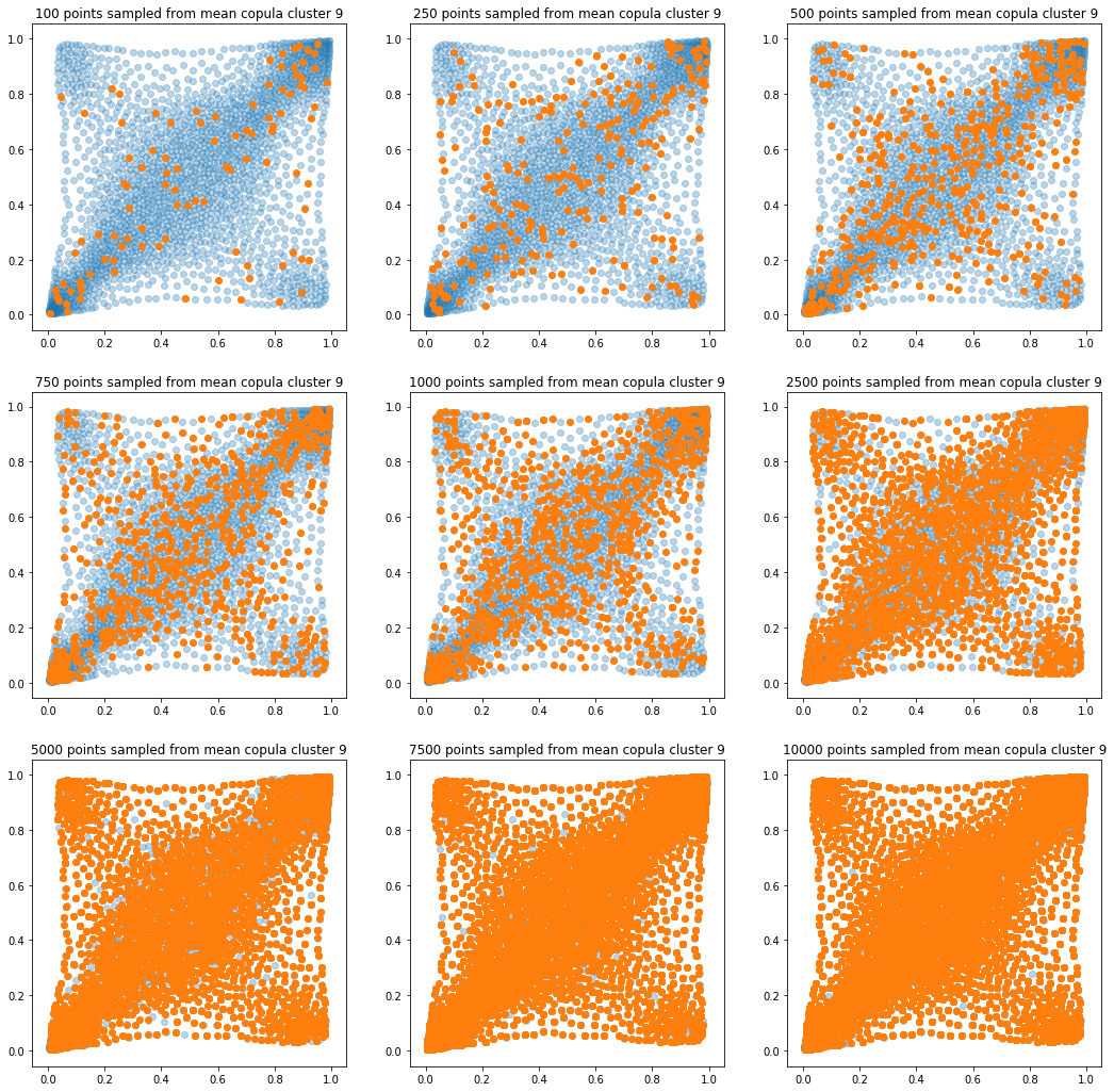
In translucent light blue, the empirical distribution (supported by 1008 ‘diracs’) from which the samples are drawn. In orange, the samples of various sizes.
sample_sizes = [100, 250, 500,
                750, 1000, 2500,
                5000, 7500, 10000]

for k in range(len(mean_copula_large_support)):
    plt.figure(figsize=(18, 18))

    for i, sample_size in enumerate(sample_sizes):
        new_u, new_v = sample_from_cdf(
            mean_copula_large_support[k], size=sample_size, nb_bins=300)

        plt.subplot(3, 3, i + 1)
        plt.scatter(mean_copula_large_support[k][:, 0],
                    mean_copula_large_support[k][:, 1],
                    alpha=0.3)
        plt.scatter(new_u, new_v)
        plt.title('{} points sampled from mean copula cluster {}'
                  .format(sample_size, k + 1))
    plt.show()
In this short blog, we proposed this simple sampling method as a baseline.
It still remains to:
- try to find stylized facts,
- explore/cluster the margins,
- sample from bivariate joint distribution of returns (using the copula and the two margins);
And, finally, create/develop/experiment with CopulaGAN.