Clustering Marginal Distributions of Stocks Returns, and Sampling from their Wasserstein Barycenter
Clustering Marginal Distributions of Stocks Returns, and Sampling from their Wasserstein Barycenter
In continuation of the previous short blogs
we do the same, but for margins.
That is,
- hierarchical clustering of margins using 1D optimal transport as a distance between the univariate distributions of stocks returns,
- summarizing these distributions with a Wasserstein barycenter per cluster,
- sampling ‘returns’ from the average margins.
Using results from the previous blogs (stocks copula, and its sampling), we can now sample from the joint bivariate distribution of stocks returns. This stems from Sklar’s theorem, and is illustrated as a conclusion to this blog.
%matplotlib inline

import pandas as pd
import numpy as np
from scipy.stats import rankdata
from scipy.cluster import hierarchy
import ot
import fastcluster
import matplotlib.pyplot as plt
df = pd.read_csv('data/SP500_HistoTimeSeries.csv')
df = df.set_index('Date')
df.index = pd.to_datetime(df.index)
df = df.sort_index()
df = df.fillna(method='ffill', limit=5)
del df['SPX Index']
returns = df.pct_change()

recent_returns = returns.iloc[-252 * 4:]

for col in recent_returns:
    try:
        if (len(recent_returns[col].dropna()) <
            len(recent_returns[col])):
            del recent_returns[col]
        if col not in industry_tickers:
            del recent_returns[col]
    except:
        pass
Below we compute $N = 478$ histograms representing the distribution of stocks returns:
histograms = {}
nb_bins = 100
for name in recent_returns.columns:
    histograms[name] = plt.hist(
        recent_returns[name].values, bins=nb_bins)
We then compute pairwise distances between all these histograms:
N = len(recent_returns.columns)
dist_mat = np.zeros((N, N))

for i, name1 in enumerate(recent_returns.columns):
    hist1 = histograms[name1]
    mid_bins1 = 0.5 * (hist1[1][:-1] + hist1[1][1:])
    for j, name2 in enumerate(recent_returns.columns):
        if j > i:
            hist2 = histograms[name2]
            mid_bins2 = 0.5 * (hist2[1][:-1] + hist2[1][1:])

            M = ot.dist(mid_bins1.reshape((nb_bins, 1)),
                        mid_bins2.reshape((nb_bins, 1)))
            M /= M.max()

            G0 = ot.emd(hist1[0] / hist1[0].sum(),
                        hist2[0] / hist2[0].sum(),
                        M)

            # compute the optimal transport distance:
            # <optimal transport matrix, ground distance matrix>_F
            ot_dist = np.trace(np.dot(np.transpose(G0), M))

            dist_mat[i, j] = ot_dist
            dist_mat[j, i] = ot_dist
From there, the usual code snippet to sort the distance matrix, and extract clusters from it:
def extract_clusters(dist, nb_clusters=3):
    dim = len(dist)
    tri_a, tri_b = np.triu_indices(dim, k=1)
    Z = fastcluster.linkage(dist[tri_a, tri_b], method='ward')
    clustering_inds = hierarchy.fcluster(Z, nb_clusters,
                                         criterion='maxclust')
    clusters = {i: [] for i in range(min(clustering_inds),
                                     max(clustering_inds) + 1)}
    for i, v in enumerate(clustering_inds):
        clusters[v].append(i)

    return clusters
dist = dist_mat
dim = len(dist)
tri_a, tri_b = np.triu_indices(dim, k=1)
Z = fastcluster.linkage(dist[tri_a, tri_b], method='ward')
permutation = hierarchy.leaves_list(
    hierarchy.optimal_leaf_ordering(Z, dist[tri_a, tri_b]))
HC_tickers = recent_returns.columns[permutation]
HC_distrib = dist_mat[permutation, :][:, permutation]

clusters = extract_clusters(HC_distrib, nb_clusters=5)

plt.pcolormesh(HC_distrib)
for cluster_id, cluster in clusters.items():
    xmin, xmax = min(cluster), max(cluster)
    ymin, ymax = min(cluster), max(cluster)

    plt.axvline(x=xmin,
                ymin=ymin / dim, ymax=(ymax + 1) / dim,
                color='r')
    plt.axvline(x=xmax + 1,
                ymin=ymin / dim, ymax=(ymax + 1) / dim,
                color='r')
    plt.axhline(y=ymin,
                xmin=xmin / dim, xmax=(xmax + 1) / dim,
                color='r')
    plt.axhline(y=ymax + 1,
                xmin=xmin / dim, xmax=(xmax + 1) / dim,
                color='r')
plt.colorbar()
plt.show()
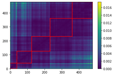
We highlight in red, in the picture just above, the 5 clusters of distributions we found.
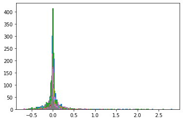
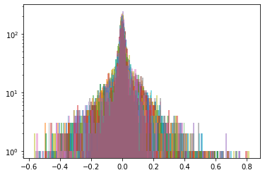
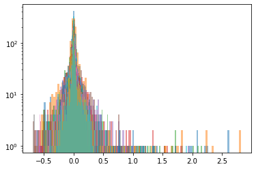
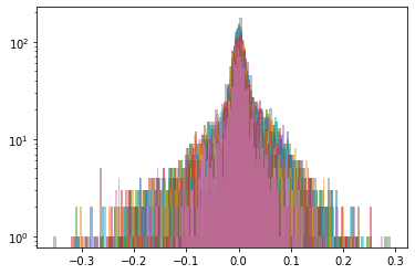
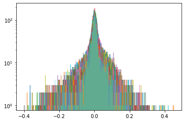
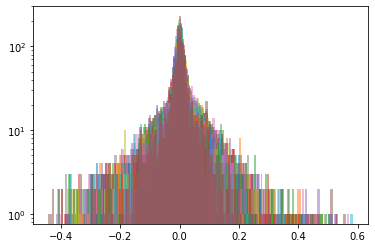
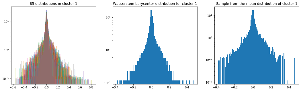
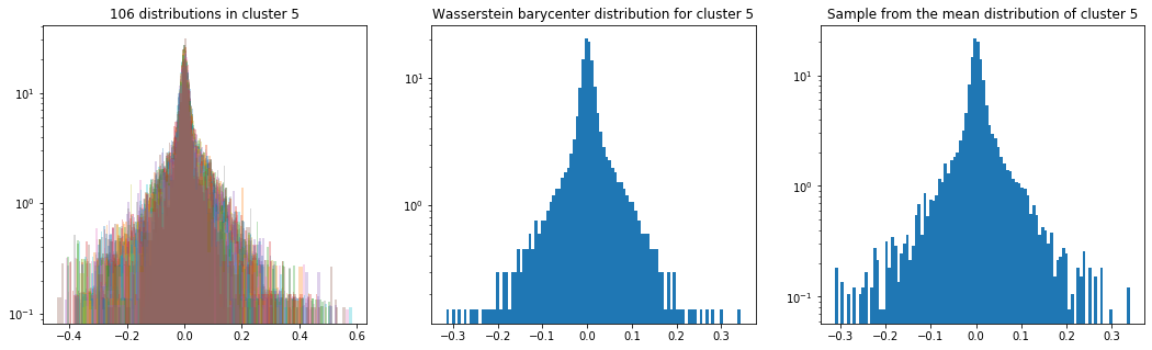
Below, we display the stocks and their distribution (in log frequency to better visualize the tails) in each cluster:
measures_cluster = {cluster: []
                    for cluster, elems in clusters.items()}

for cluster, elems in clusters.items():
    print('Cluster {}'.format(cluster))
    print(HC_tickers[elems])
    rets = recent_returns[HC_tickers[elems]]

    for c in rets.columns:
        measures_cluster[cluster].append(
            {'locations': rets[c].values,
             'weights': np.ones(len(rets[c])) / len(rets[c])})
        plt.hist(rets[c].values,
                 bins=nb_bins, log=True, alpha=0.5)
    plt.show()
Cluster 1
Index(['MLM UN Equity', 'ALB UN Equity', 'SEE UN Equity', 'LNC UN Equity',
       'ADS UN Equity', 'EQIX UW Equity', 'LB UN Equity', 'LYB UN Equity',
       'LM UN Equity', 'TSN UN Equity', 'GPN UN Equity', 'LVLT UN Equity',
       'HCA UN Equity', 'CRM UN Equity', 'HUM UN Equity', 'RCL UN Equity',
       'AYI UN Equity', 'PHM UN Equity', 'PBI UN Equity', 'ETFC UW Equity',
       'EXPE UW Equity', 'PCLN UW Equity', 'CELG UW Equity', 'BSX UN Equity',
       'HBI UN Equity', 'GILD UW Equity', 'ATVI UW Equity', 'AGN UN Equity',
       'AMZN UW Equity', 'LUV UN Equity', 'UA UN Equity', 'DAL UN Equity',
       'EW UN Equity', 'NVDA UW Equity', 'ULTA UW Equity', 'XEC UN Equity',
       'CNC UN Equity', 'AVGO UW Equity', 'UAL UN Equity', 'ALK UN Equity',
       'URI UN Equity', 'IRM UN Equity', 'CMG UN Equity', 'MNST UW Equity',
       'CXO UN Equity', 'AMAT UW Equity', 'YHOO UW Equity', 'PXD UN Equity',
       'MYL UW Equity', 'HAR UN Equity', 'MPC UN Equity', 'VLO UN Equity',
       'SPLS UW Equity', 'AKAM UW Equity', 'HES UN Equity', 'OI UN Equity',
       'FFIV UW Equity', 'ALXN UW Equity', 'CTL UN Equity', 'ADSK UW Equity',
       'CF UN Equity', 'GRMN UW Equity', 'PVH UN Equity', 'BWA UN Equity',
       'STJ UN Equity', 'ISRG UW Equity', 'WHR UN Equity', 'SIG UN Equity',
       'BIIB UW Equity', 'EQT UN Equity', 'APC UN Equity', 'NBL UN Equity',
       'FTR UW Equity', 'HAL UN Equity', 'VIAB UW Equity', 'HRB UN Equity',
       'STZ UN Equity', 'TDC UN Equity', 'FMC UN Equity', 'MOS UN Equity',
       'COH UN Equity', 'NOV UN Equity', 'KSS UN Equity', 'R UN Equity',
       'M UN Equity'],
      dtype='object')
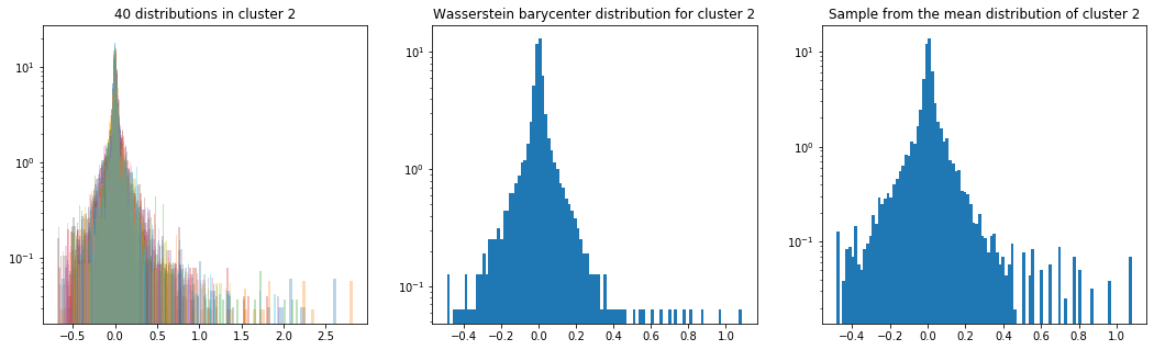
Cluster 2
Index(['ENDP UW Equity', 'CHK UN Equity', 'SWN UN Equity', 'FCX UN Equity',
       'FSLR UW Equity', 'NFLX UW Equity', 'MU UW Equity', 'BBY UN Equity',
       'RIG UN Equity', 'WYNN UW Equity', 'NRG UN Equity', 'KMI UN Equity',
       'VRTX UW Equity', 'OKE UN Equity', 'RRC UN Equity', 'STX UW Equity',
       'NEM UN Equity', 'MUR UN Equity', 'KORS UN Equity', 'MRO UN Equity',
       'FB UW Equity', 'HP UN Equity', 'APA UN Equity', 'DVN UN Equity',
       'WDC UW Equity', 'COG UN Equity', 'WMB UN Equity', 'HPQ UN Equity',
       'DO UN Equity', 'URBN UW Equity', 'WFM UW Equity', 'AA UN Equity',
       'GPS UN Equity', 'SWKS UW Equity', 'REGN UW Equity', 'TSO UN Equity',
       'NFX UN Equity', 'ILMN UW Equity', 'EA UW Equity', 'TRIP UW Equity'],
      dtype='object')
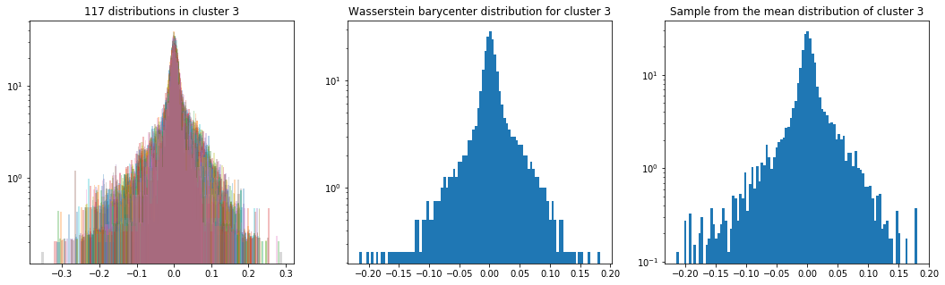
Cluster 3
Index(['FAST UW Equity', 'MSI UN Equity', 'WAT UN Equity', 'EXPD UW Equity',
       'COL UN Equity', 'AEE UN Equity', 'WEC UN Equity', 'LLTC UW Equity',
       'JPM UN Equity', 'NTRS UW Equity',
       ...
       'KO UN Equity', 'PM UN Equity', 'K UN Equity', 'USB UN Equity',
       'SO UN Equity', 'PBCT UW Equity', 'MTB UN Equity', 'D UN Equity',
       'PPL UN Equity', 'TROW UW Equity'],
      dtype='object', length=117)
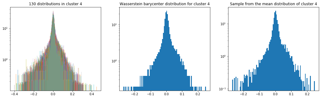
Cluster 4
Index(['SCG UN Equity', 'KIM UN Equity', 'GS UN Equity', 'CCL UN Equity',
       'ADI UW Equity', 'DRI UN Equity', 'IFF UN Equity', 'MDLZ UW Equity',
       'OMC UN Equity', 'GWW UN Equity',
       ...
       'INTU UW Equity', 'NI UN Equity', 'ESRX UW Equity', 'LLY UN Equity',
       'APH UN Equity', 'BDX UN Equity', 'HSIC UW Equity', 'ITW UN Equity',
       'APD UN Equity', 'GPC UN Equity'],
      dtype='object', length=130)
Cluster 5
Index(['WU UN Equity', 'ICE UN Equity', 'PRU UN Equity', 'INTC UW Equity',
       'LEN UN Equity', 'BA UN Equity', 'NOC UN Equity', 'PFG UN Equity',
       'AMP UN Equity', 'SBUX UW Equity',
       ...
       'SE UN Equity', 'UNP UN Equity', 'DD UN Equity', 'RL UN Equity',
       'AES UN Equity', 'JWN UN Equity', 'BBBY UW Equity', 'KLAC UW Equity',
       'CMI UN Equity', 'DLR UN Equity'],
      dtype='object', length=106)
def sample_from_ecdf_1d(margin, size=500, nb_bins=100):
    hist, bins = np.histogram(margin, bins=nb_bins)
    bin_midpoints = bins[:-1] + np.diff(bins) / 2
    cdf = np.cumsum(hist)
    cdf = cdf / cdf[-1]
    values = np.random.uniform(size=size)
    value_bins = np.searchsorted(cdf, values)
    random_from_cdf = bin_midpoints[value_bins]

    return random_from_cdf
As in the previous blog, we compute the Wasserstein barycenter of the distributions (per cluster), and then we sample from this average distribution for illustration purpose.
Plots of the distributions are in log density.
barycenter_distribution = {}
for cluster, elems in clusters.items():

    print('Cluster {}'.format(cluster))
    rets = recent_returns[HC_tickers[elems]]

    size, nb_distributions = rets.shape
    X_init = np.random.uniform(size=size)
    X_init = X_init.reshape((len(rets), 1))

    k = size
    b = np.ones((k,)) / k

    locations = [measures_cluster[cluster][idx]['locations']
                 .reshape((len(rets), 1))
                 for idx in range(nb_distributions)]
    weights = [measures_cluster[cluster][idx]['weights']
               for idx in range(nb_distributions)]

    X = ot.lp.free_support_barycenter(
        locations, weights, X_init, b)

    barycenter_distribution[cluster] = X

    plt.figure(figsize=(18, 5))

    plt.subplot(1, 3, 1)
    for c in rets.columns:
        plt.hist(rets[c].values, bins=nb_bins,
                 log=True, density=True, alpha=0.3)
    plt.title('{} distributions in cluster {}'
              .format(nb_distributions, cluster))

    plt.subplot(1, 3, 2)
    plt.hist(barycenter_distribution[cluster], bins=nb_bins,
             log=True, density=True)
    plt.title('Wasserstein barycenter distribution for cluster {}'
              .format(cluster))

    random_from_cdf = sample_from_ecdf_1d(
        barycenter_distribution[cluster],
        size=size * 10,
        nb_bins=nb_bins)

    hist, bins = np.histogram(X, bins=nb_bins)
    bin_midpoints = bins[:-1] + np.diff(bins) / 2
    cdf = np.cumsum(hist)
    cdf = cdf / cdf[-1]
    values = np.random.uniform(size=size * 10)
    value_bins = np.searchsorted(cdf, values)
    random_from_cdf = bin_midpoints[value_bins]

    plt.subplot(1, 3, 3)
    plt.hist(random_from_cdf, bins=nb_bins,
             log=True, density=True)
    plt.title('Sample from the mean distribution of cluster {}'
              .format(cluster))

    plt.show()
Cluster 1
Cluster 2
Cluster 3
Cluster 4
Cluster 5
That’s it for the margins.
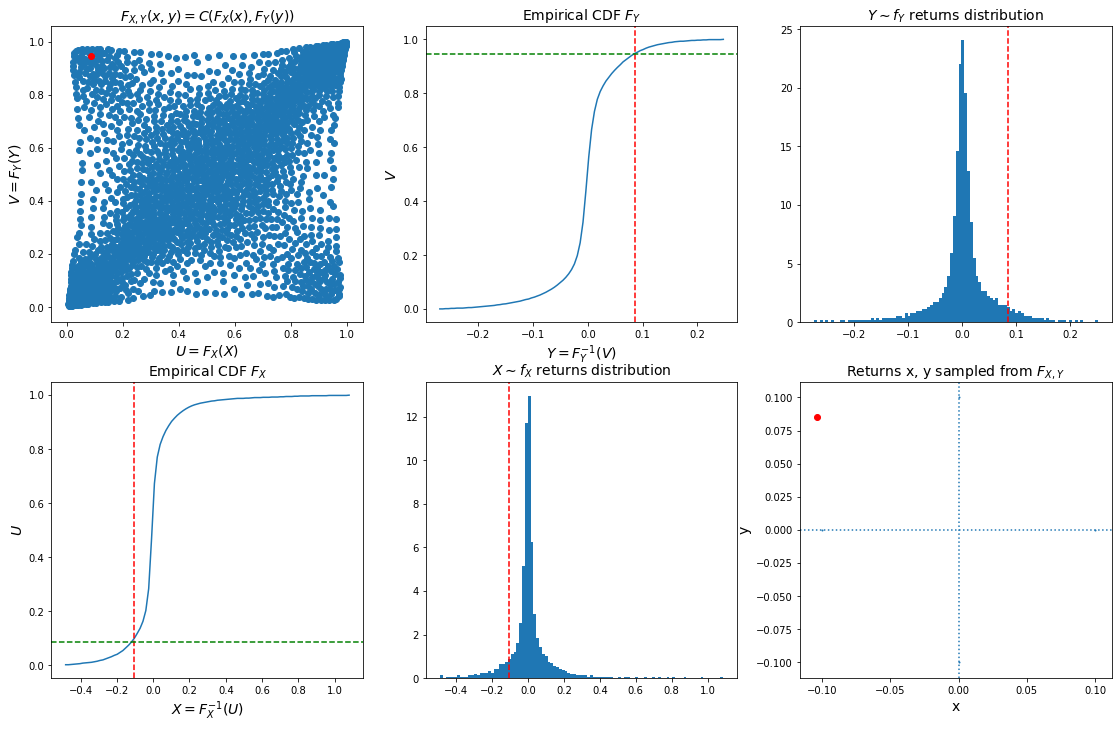
As a conclusion, we can now sample from the joint bivariate distribution of stocks returns using a copula (pre-computed in previous blog Wasserstein Barycenters of Stocks Empirical Copulas), the margins computed above, and Sklar’s theorem $F_{X, Y}(x, y) = C(F_X(x), F_Y(y))$.
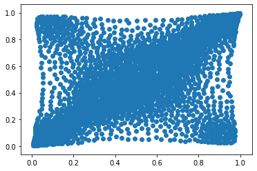
Let’s load and display a bivariate copula of stocks returns.
copula_model = np.load('mean_copula_large_support_cluster_0.npy')
plt.scatter(copula_model[:, 0], copula_model[:, 1])
plt.show()
Let’s define inverse probability integral transforms for the copula, and the margins:
- sample a random point $(u, v)$ from the copula,
- invert the margins: $x = F_X^{-1}(u)$, $y = F_Y^{-1}(v)$
def inversion_sampling_ecdf_1d(margin, values, nb_bins=100):
    hist, bins = np.histogram(margin, bins=nb_bins)
    bin_midpoints = bins[:-1] + np.diff(bins) / 2
    cdf = np.cumsum(hist)
    cdf = cdf / cdf[-1]
    value_bins = np.searchsorted(cdf, values)
    random_from_cdf = bin_midpoints[value_bins]

    return random_from_cdf

def sample_from_ecdf_2d(margins, size=500, nb_bins=100):
    hist, x_bins, y_bins = np.histogram2d(
        margins[:, 0], margins[:, 1], bins=(nb_bins, nb_bins))
    x_bin_midpoints = x_bins[:-1] + np.diff(x_bins) / 2
    y_bin_midpoints = y_bins[:-1] + np.diff(y_bins) / 2

    cdf = np.cumsum(hist.ravel())
    cdf = cdf / cdf[-1]

    values = np.random.uniform(size=size)
    value_bins = np.searchsorted(cdf, values)

    x_idx, y_idx = np.unravel_index(
        value_bins, (len(x_bin_midpoints), len(y_bin_midpoints)))

    random_from_cdf = np.column_stack(
        (x_bin_midpoints[x_idx], y_bin_midpoints[y_idx]))
    new_x, new_y = random_from_cdf.T

    return new_x, new_y
u, v = sample_from_ecdf_2d(copula_model, size=1, nb_bins=300)
x = inversion_sampling_ecdf_1d(barycenter_distribution[2], u, nb_bins=100)
y = inversion_sampling_ecdf_1d(barycenter_distribution[4], v, nb_bins=100)
plt.figure(figsize=(19, 12))

plt.subplot(2, 3, 1)
plt.scatter(copula_model[:, 0], copula_model[:, 1])
plt.scatter([u], [v], color='r')
plt.xlabel('$U = F_X(X)$', fontsize=14)
plt.ylabel('$V = F_Y(Y)$', fontsize=14)
plt.title('$F_{X, Y}(x, y) = C(F_X(x), F_Y(y))$', fontsize=14)


hy = np.histogram(barycenter_distribution[4], bins=nb_bins)

plt.subplot(2, 3, 2)
cdf = np.cumsum(hy[0])
cdf = cdf / cdf[-1]
plt.plot(hy[1][:-1] + np.diff(hy[1]) / 2, cdf)
plt.axvline(x=y, linestyle='dashed', color='red')
plt.axhline(y=v, linestyle='dashed', color='green')
plt.ylabel('$V$', fontsize=14)
plt.xlabel('$Y = F_Y^{-1}(V)$', fontsize=14)
plt.title('Empirical CDF $F_Y$', fontsize=14)

plt.subplot(2, 3, 3)
plt.hist(barycenter_distribution[4],
         bins=nb_bins, density=True)
plt.axvline(x=y, linestyle='dashed', color='red')
plt.title('$Y \sim f_Y$ returns distribution',
          fontsize=14)


hx = np.histogram(barycenter_distribution[2], bins=nb_bins)

plt.subplot(2, 3, 4)
cdf = np.cumsum(hx[0])
cdf = cdf / cdf[-1]
plt.plot(hx[1][:-1] + np.diff(hx[1]) / 2, cdf)
plt.axvline(x=x, linestyle='dashed', color='red')
plt.axhline(y=u, linestyle='dashed', color='green')
plt.ylabel('$U$', fontsize=14)
plt.xlabel('$X = F_X^{-1}(U)$', fontsize=14)
plt.title('Empirical CDF $F_X$', fontsize=14)

plt.subplot(2, 3, 5)
plt.hist(barycenter_distribution[2],
         bins=nb_bins, density=True)
plt.axvline(x=x, linestyle='dashed', color='red')
plt.title('$X \sim f_X$ returns distribution',
          fontsize=14)


plt.subplot(2, 3, 6)
val = 0.1
plt.scatter([-val, val, 0, 0], [0, 0, -val, val], s=1)
plt.scatter([x], [y], color='r')
plt.axvline(x=0, linestyle='dotted')
plt.axhline(y=0, linestyle='dotted')
plt.title(r'Returns x, y sampled from $F_{X, Y}$',
          fontsize=14)
plt.xlabel('x', fontsize=14)
plt.ylabel('y', fontsize=14)

plt.show()
Conclusion: In this blog, we illustrated how to use copula and margins to sample from a joint distribution.
We did so after exploring what were typical (univariate) distributions of stocks returns using tools such as optimal transport and clustering.
However, we did this exploration without taking into consideration the dependence structure (say correlation) between stocks. A next step would be to consider both the dependence structure and the distribution of returns when clustering stocks.
That would maybe allow us to develop a hierarchical model for simulations having a mean copula and a mean marginal per cluster; inter-clusters it could be the copula between their respective ‘first factor’. This hierarchical model could be put in competition with CopulaGAN, or complement it. To be seen…