How to combine a handful of predictors using empirical copulas and maximum likelihood
How to combine a handful of predictors using empirical copulas and maximum likelihood
In this blog, I will present another empirical copula trick for combining a handful of forecasters. Each forecaster can have its own bias with different levels of noise. The copula is useful to learn and leverage the potentially non-linear correlations existing between the forecasters errors.
Note that a similar idea was presented in Copulas-based time series combined forecasters. However, authors use a Gumbel-Hougaard copula which can only capture positive dependence (forecasters cannot have anti-correlated errors). Using an empirical copula instead allows for all possible dependence structure between the forecasters errors. Restriction to a handful of predictors (low dimension) is the trade-off for this added expressive power.
This copula-based method can shine when there are complex (but stable) non-linear correlations between the forecasters errors. On the contrary, a linear regression would suffer from the potentially high correlations between the errors.
There are many possible ways to combine predictions. Some are based on:
- measures of ‘centrality’ of the distribution of predictions (e.g. mean, median)
- linear regressions,
- bagging,
- boosting,
- stacking, i.e. applying yet another model on top of the predictions produced by a previous layer of models.
This is not the goal here to perform an exhaustive comparison of all these methods.
%matplotlib inline

import numpy as np
import pandas as pd
import scipy
from scipy.stats import rankdata
from statsmodels.tsa.arima_model import ARMA
from statsmodels.tsa.arima_process import arma_generate_sample
import matplotlib.pyplot as plt
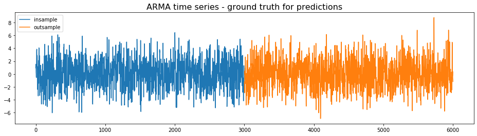
We generate an ARMA time series, which will be considered the ground truth for the predictions. The first half will be used for the training, the second half for the testing.
import numpy as np

arparams = np.array([.75, -.25])
maparams = np.array([.65, .35])

ar = np.r_[1, -arparams]
ma = np.r_[1, maparams]

T = 3000
insample = arma_generate_sample(ar, ma, T)
insample = pd.Series(insample, index=range(0, T))
outsample = arma_generate_sample(ar, ma, T)
outsample = pd.Series(outsample, index=range(T, 2 * T))

model = ARMA(insample, (2, 2)).fit(trend='nc', disp=0)
model.params
ar.L1.y    0.742088
ar.L2.y   -0.250448
ma.L1.y    0.651244
ma.L2.y    0.342461
dtype: float64
plt.figure(figsize=(16, 4))
plt.plot(insample, label='insample')
plt.plot(outsample, label='outsample')
plt.legend()
plt.title('ARMA time series - ground truth for predictions',
          fontsize=16)
plt.show()
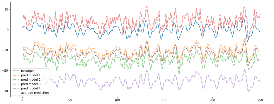
To illustrate the copula-based approach, we will use dummy models: the prediction of the next value = the current value + some idiosyncratic i.i.d. noise with a given bias and variance.
Since all the predictors are based on the last observed value, they are correlated to some extent. Their correlation strength is determined by their i.i.d. noise: the higher the noise variance, the less correlated they are with other predictors.
biases = [-10, -15, 4, -25]
scales = [0.1, 1, 2, 0.2]

models = [insample.shift(1) +
          np.random.normal(loc=biases[i], scale=scales[i], size=T)
          for i in range(len(biases))]

nb_models = len(models)

average_model = pd.DataFrame(np.array(models).T).mean(axis=1)
We can see the different biases and variances of the 4 models. We only show the first 250 points of the time series below:
max_steps = 250
plt.figure(figsize=(16, 6))
plt.plot(insample.loc[:max_steps], label='insample')
for idx, model in enumerate(models):
    plt.plot(model.loc[:max_steps], '--', linewidth=3, alpha=0.5,
             label='pred model {}'.format(idx + 1))
plt.plot(average_model.loc[:max_steps], linewidth=1,
         label='average prediction')
plt.legend()
plt.show()
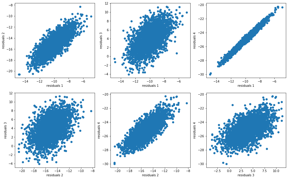
For each model, we compute the residuals:
model_residuals = [model - insample for model in models]
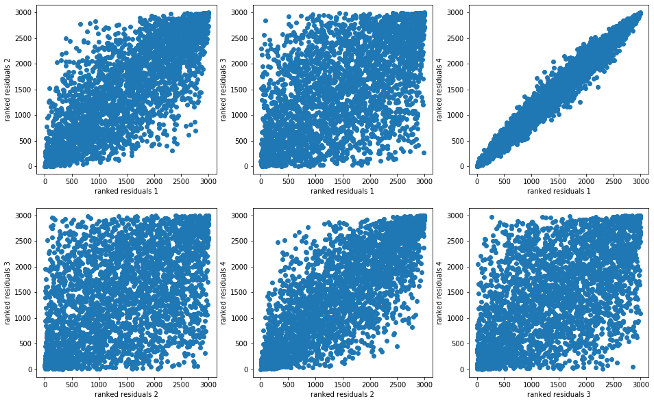
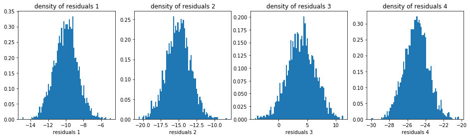
And we display their distributions (joint distributions, dependence structure, marginals):
nb_bins_4d = 7
nb_bins_1d = 80

plt.figure(figsize=(16, 10))
idx = 1
for i in range(nb_models):
    for j in range(nb_models):
        if j > i:
            plt.subplot(2, 3, idx)
            plt.scatter(model_residuals[i], model_residuals[j])
            plt.xlabel(f"residuals {i + 1}")
            plt.ylabel(f"residuals {j + 1}")
            idx += 1
plt.show()

plt.figure(figsize=(16, 10))
idx = 1
for i in range(nb_models):
    for j in range(nb_models):
        if j > i:
            plt.subplot(2, 3, idx)
            plt.scatter(rankdata(model_residuals[i]),
                        rankdata(model_residuals[j]))
            plt.xlabel(f"ranked residuals {i + 1}")
            plt.ylabel(f"ranked residuals {j + 1}")
            idx += 1
plt.show()

r = (pd.DataFrame(np.array(model_residuals).T)
     .dropna()
     .rank(axis=0)
     .values)
density, edges = np.histogramdd(r, density=True, bins=nb_bins_4d)

plt.figure(figsize=(16, 4))
idx = 1
u_densities = []
u_edges = []
for i in range(nb_models):
    plt.subplot(1, 4, idx)
    # compute the density (via binning) of the residuals of model i
    d, e = np.histogram(model_residuals[i].dropna(),
                        density=True, bins=nb_bins_1d)
    u_densities.append(d)
    u_edges.append(e)
    plt.hist(model_residuals[i].dropna(), density=True, bins=nb_bins_1d)
    plt.xlabel(f'residuals {i + 1}')
    plt.title(f'density of residuals {i + 1}')
    idx += 1
plt.show()
Based on this information, we will compute the value $v$ which maximizes the likelihood of the errors (= predictions - $v$) distribution. This maximum likelihood estimate $v$ is the copula-based combined forecasters prediction.
def predict_using_copula(model_preds, insample,
                         disp=False, grid_size=1000):
    grid = np.linspace(min(insample.min(),
                           min([model.min() for model in models])),
                       max(insample.max(),
                           max([model.max() for model in models])),
                       num=grid_size)

    nb_predictors = len(model_preds)
    ml = np.zeros(grid_size)
    for idx_grid, val_grid in enumerate(grid):
        ranks = []
        residuals = []
        for idx_pred in range(nb_predictors):
            val_model = model_preds[idx_pred]
            residual = val_model - val_grid
            residuals.append(residual)

            model_residuals[idx_pred].loc[0] = residual
            rk = model_residuals[idx_pred].rank()[0]
            ranks.append(rk)

        c = density[tuple([[min(np.searchsorted(e, r) - 1, nb_bins_4d - 1)]
                           for e, r in zip(edges, ranks)])][0]

        p = [d[min(np.searchsorted(e, r) - 1, nb_bins_1d - 1)]
             for r, d, e in zip(residuals, u_densities, u_edges)]

        ml[idx_grid] = c * np.prod(p)

    if disp:
        plt.plot(ml)
        plt.show()

    return grid[ml.argmax()]
Let’s apply it on an example. Given the value observed at time $t$, and 4 forecasts for $t + 1$, we obtain the copula-based prediction for $t + 1$:
cur_t = T
ground_truth = outsample.loc[cur_t + 1]

cur_value = outsample.loc[cur_t]
model_preds = [cur_value + np.random.normal(loc=biases[i], scale=scales[i])
               for i in range(len(biases))]
final_prediction = predict_using_copula(model_preds, insample, disp=True)
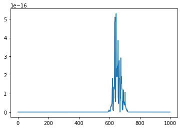
The final prediction is the one which maximizes the likelihood.
The copula-based prediction is the closest one to the ground truth value at $t + 1$:
print('value at time t:\t\t', round(cur_value, 3),
 '\nprediction model 1 for t + 1:\t', round(model_preds[0], 3),
 '\nprediction model 2 for t + 1:\t', round(model_preds[1], 3),
 '\nprediction model 3 for t + 1:\t', round(model_preds[2], 3),
 '\nprediction model 4 for t + 1:\t', round(model_preds[3], 3),
 '\naverage prediction for t + 1:\t', round(np.mean(model_preds), 3),
 '\ncopula prediction for t + 1:\t', round(final_prediction, 3),
 '\nground truth at t + 1:\t\t', round(ground_truth, 3))
value at time t:		 -1.238
prediction model 1 for t + 1:	 -11.325
prediction model 2 for t + 1:	 -15.871
prediction model 3 for t + 1:	 1.807
prediction model 4 for t + 1:	 -26.112
average prediction for t + 1:	 -12.875
copula prediction for t + 1:	 -1.701
ground truth at t + 1:		 -2.517
We do the same for the next 250 steps:
average_predictions = []
copula_predictions = []
true_values = []
all_preds = []
for cur_t in range(T, T + max_steps):
    cur_value = outsample.loc[cur_t]
    model_preds = [cur_value + np.random.laplace(loc=biases[i], scale=scales[i])
                   for i in range(len(biases))]

    final_prediction = predict_using_copula(model_preds, insample, disp=False)

    copula_predictions.append(final_prediction)
    average_predictions.append(np.mean(model_preds))
    true_values.append(outsample.loc[cur_t + 1])
    all_preds.append(model_preds)
model_predictions = np.array(all_preds)
plt.figure(figsize=(16, 6))
plt.plot(true_values,
'-o', color='blue', label='out-of-sample')
for i in range(model_predictions.shape[1]):
plt.plot(model_predictions[:, i],
alpha=0.6, label='model {} preds'.format(i + 1))
plt.plot(copula_predictions,
'-o', color='green', label='copula predictions')
plt.plot(average_predictions,
'--', color='black', label='average predictions')
plt.legend(fontsize=14)
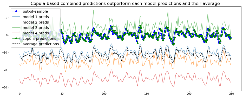
plt.title('Copula-based combined predictions outperform ' +
'each model predictions and their average', fontsize=16)
plt.show()
We observe that the copula-based forecaster does consistently better than the individual models, or their average forecast.
Conclusion: In this blog post, we have illustrated an idea for combining forecasts based on empirical copulas which is little known from the machine learning crowd. We showed on a simple example (ARMA time series and dummy predictors) that this approach could effectively combined a handful of forecasts. This method should work very well as long as the distribution of errors remains stable.
The regression problem exposed here was overly simplistic. In subsequent studies we shall see whether this copula-based approach can consistently outperform other combination methods.
Thanks to Tomas Thornquist for proofreading and suggesting for further studies more realistic simulations.