Portfolio construction methods and risk metrics: in- and out-of-sample comparisons on simulated data
Portfolio construction methods and risk metrics: in- and out-of-sample comparisons on simulated data
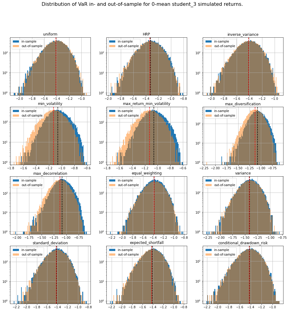
In this short blog, which is an intermediary step for more studies, we simulate data using a 0-mean multivariate Gaussian and $t$-distribution with 3 degrees of freedom both parameterized with an empirical correlation matrix used as the correlation model.
From these distributions, we build two samples of $80 \times 500$ observations (approximately two years of daily returns for 80 stocks) each:
- an in-sample dataset used to estimate an empirical covariance matrix fed to a portfolio allocation method which returns weights,
- an out-of-sample dataset on which the weights previously computed are applied; risk metrics are then computed on the resulting portfolio returns.
As for risk metrics, we will compute:
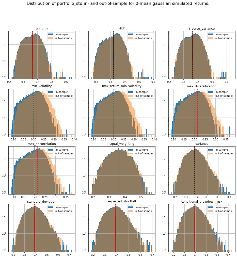
- portfolio volatility,
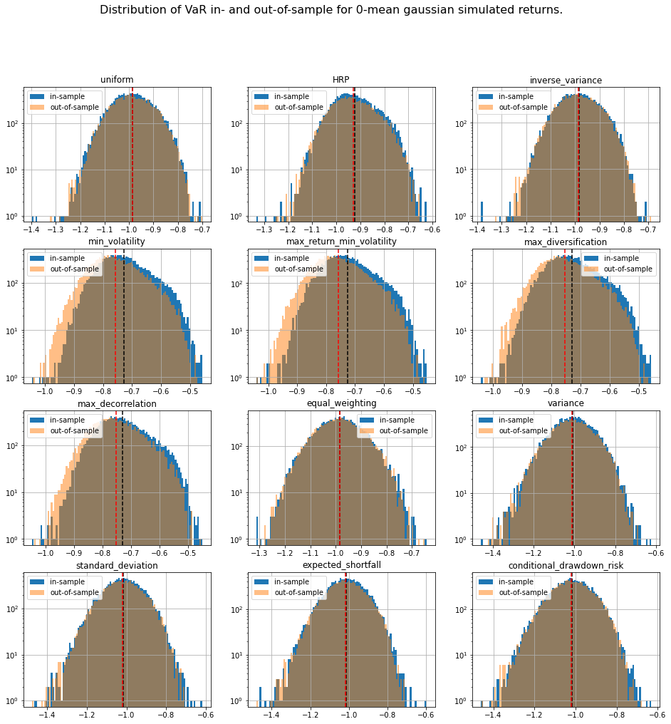
- portfolio value at risk (VaR),
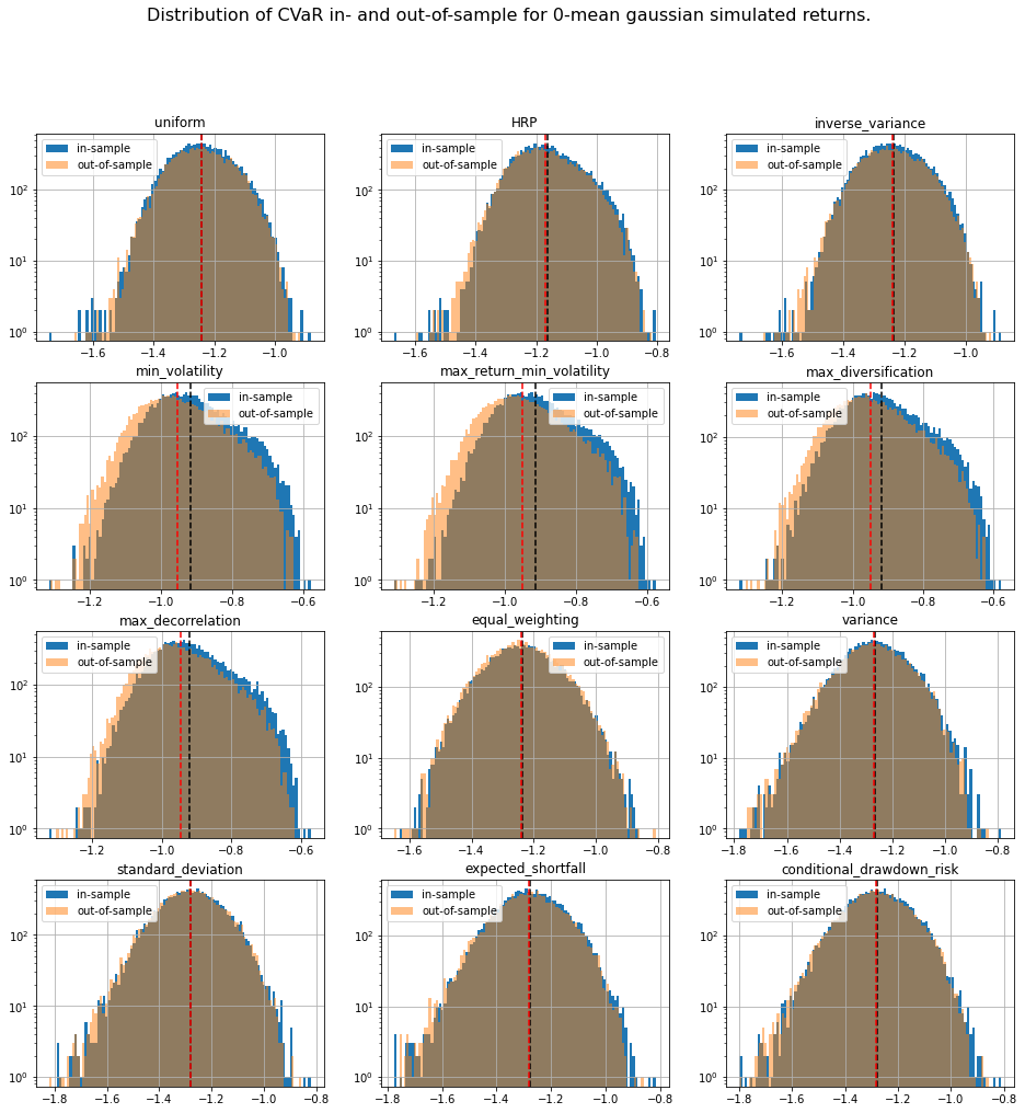
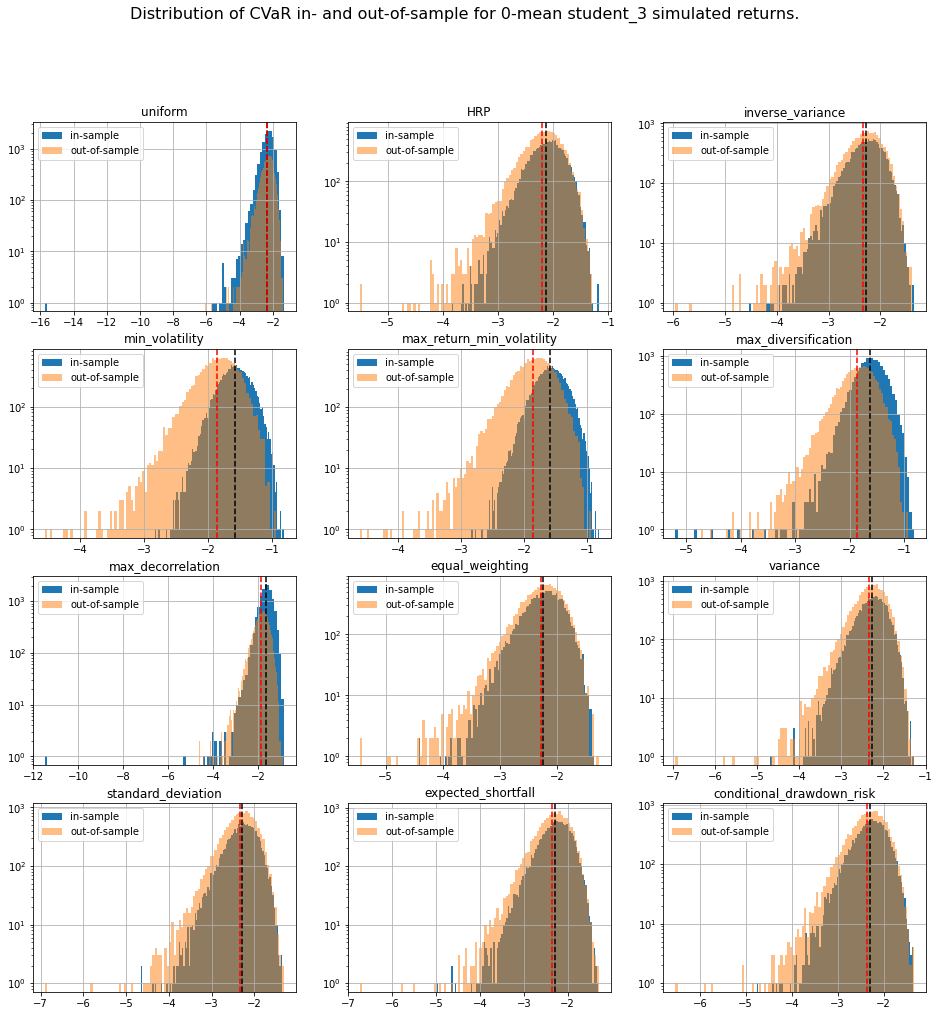
- portfolio expected shortfall (ES or CVaR),
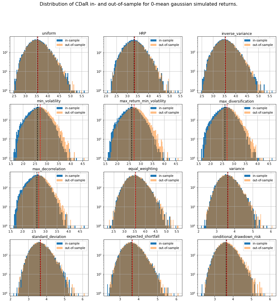
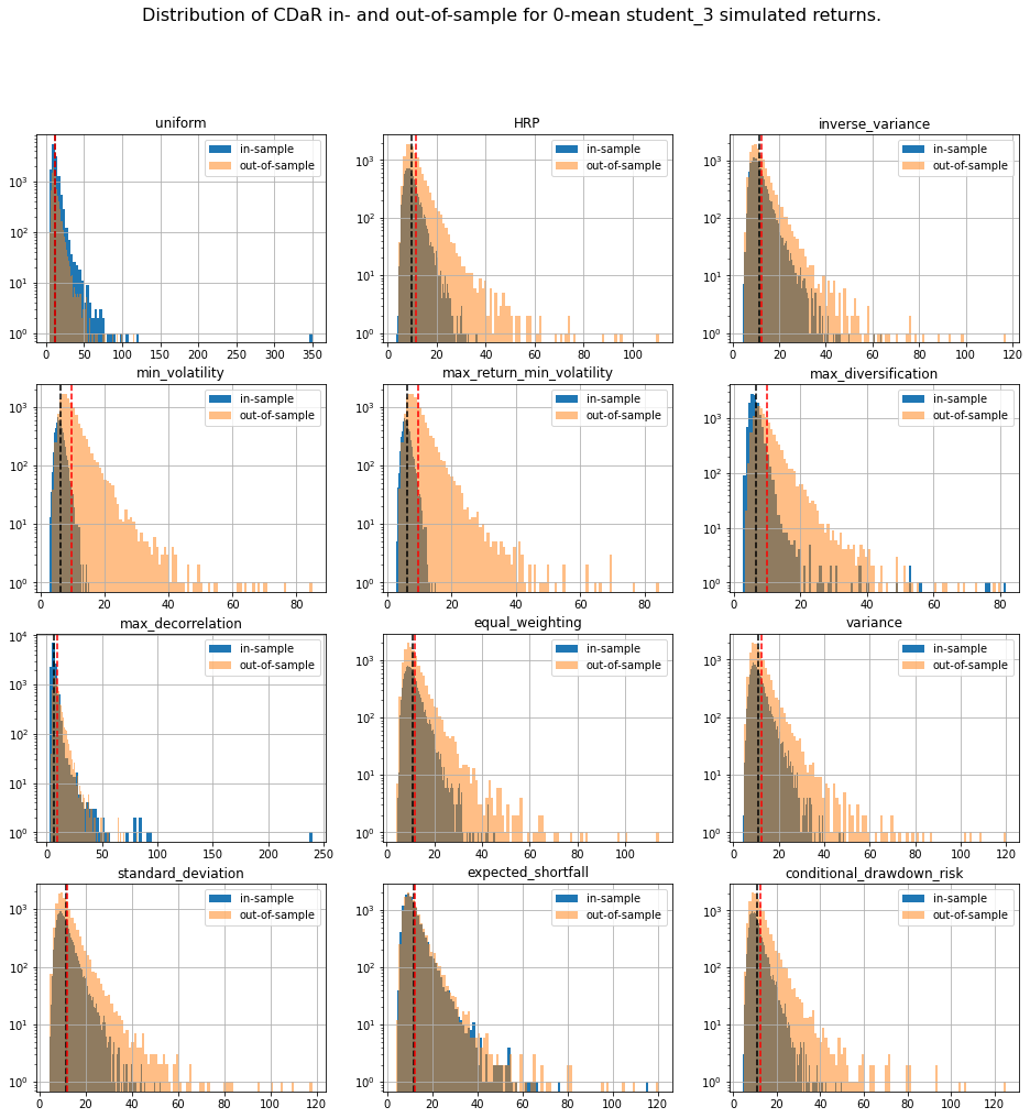
- portfolio conditional drawdown-at-risk (CDaR).
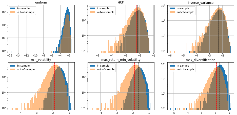
TL;DR We can notice that methods based on solving an optimization program (mean-variance style) are particularly unstable with a generally worse outcome on the out-of-sample data despite everything being the same up to some statistical noise due to finite sampling. This means that these widely used methods are unreliable on realistically sized samples, and are prone to overfitting. In this case, such methods are trying to leverage the fact that estimated vols and expected returns are not the same based on the in-sample data to find the best portfolio-solution possible; However, all vols and expected returns are actually equal.
%matplotlib inline

import numpy as np
import pandas as pd
import fastcluster
from scipy.cluster import hierarchy
from mlfinlab.portfolio_optimization import RiskMetrics
from mlfinlab.portfolio_optimization.hrp import HierarchicalRiskParity
from mlfinlab.portfolio_optimization.herc import (
    HierarchicalEqualRiskContribution)
from mlfinlab.portfolio_optimization.mean_variance import (
    MeanVarianceOptimisation)
import matplotlib.pyplot as plt
import warnings
warnings.filterwarnings("ignore")
Many portfolio allocation methods have been implemented in the Machine Learning Financial Laboratory (mlfinlab) library. I will use some of them. Very convenient.
These guys are looking for sponsorship. If you want to help them, it’s here btw.
def compute_weights(returns, cov, method='uniform'):
    if method == 'uniform':
        weights = np.ones(returns.shape[1]) / returns.shape[1]
    elif method == 'HRP':
        hrp = HierarchicalRiskParity()
        hrp.allocate(asset_names=cov.index,
                     covariance_matrix=cov)
        weights = np.array(
            [hrp.weights[col].values[0] for col in cov.index])
    elif method in ['inverse_variance', 'min_volatility',
                  'max_return_min_volatility', 'max_diversification',
                  'max_decorrelation']:
        mvo = MeanVarianceOptimisation()
        mvo.allocate(expected_asset_returns=returns.mean(axis=0),
                     covariance_matrix=cov,
                     solution=method)
        weights = np.array(mvo.weights).flatten()
        weights = np.array(mvo.weights).flatten()
    elif method in ['equal_weighting', 'variance', 'standard_deviation',
                  'expected_shortfall', 'conditional_drawdown_risk']:
        herc = HierarchicalEqualRiskContribution()
        herc.allocate(asset_returns=returns,
                      asset_names=cov.index,
                      covariance_matrix=cov,
                      risk_measure=method)
        weights = np.array(
            [herc.weights[col].values[0] for col in cov.index])
    else:
        print('Unknown method.')

    return weights
And, here, I compute a few risk metrics (still using mlfinlab):
def compute_risk_measures(returns, weights, alpha=0.05):
    portfolio_rets = np.dot(returns, weights)

    risk_met = RiskMetrics()
    portfolio_std = np.std(portfolio_rets)**2
    VaR = risk_met.calculate_value_at_risk(portfolio_rets, alpha)
    CVaR = risk_met.calculate_expected_shortfall(portfolio_rets, alpha)
    CDaR = risk_met.calculate_conditional_drawdown_risk(portfolio_rets, alpha)

    return [portfolio_std, VaR, CVaR, CDaR]
Definition of a multivariate $t$-distribution:
def multivariate_t(mean, cov, dof=3, size=500):
    dim = len(cov)
    g = np.tile(np.random.gamma(dof / 2., 2. / dof, size), (dim, 1)).T
    Z = np.random.multivariate_normal(np.zeros(dim), cov, size)
    return mean + Z / np.sqrt(g)
Loading $80 \times 80$ empirical correlation matrices which were estimated before:
matrices = np.load('empirical_matrices.npy')
Below, the core of the code:
- Generating in- and out-of-sample datasets from a distribution parameterized by the model correlation matrix;
- estimating an empirical covariance matrix on the in-sample data,
- feeding the in-sample information to an asset allocation method to get portfolio weights,
- then computing the portfolio returns and their associated risk metrics.
methods = ['uniform', 'HRP', 'inverse_variance', 'min_volatility',
           'max_return_min_volatility', 'max_diversification',
           'max_decorrelation',
           'equal_weighting', 'variance', 'standard_deviation',
           'expected_shortfall', 'conditional_drawdown_risk']

method_in_sample_risk = {method: [] for method in methods}
method_out_sample_risk = {method: [] for method in methods}

for idx_mat in range(len(matrices)):

    model_corr = matrices[idx_mat, :, :]

    in_sample = multivariate_t(mean=[0] * len(model_corr), cov=model_corr)
    in_sample = pd.DataFrame(
        in_sample, columns=['a' + str(i) for i in range(len(model_corr))])

    out_sample = multivariate_t(mean=[0] * len(model_corr), cov=model_corr)
    out_sample = pd.DataFrame(out_sample)

    assets_cov = pd.DataFrame(in_sample).cov()

    for method in methods:

        weights = compute_weights(in_sample, assets_cov, method=method)

        in_sample_risk = compute_risk_measures(in_sample, weights)
        out_sample_risk = compute_risk_measures(out_sample, weights)

        method_in_sample_risk[method].append(in_sample_risk)
        method_out_sample_risk[method].append(out_sample_risk)
We save the results (risk metrics for a given model correlation matrix) for future experiments:
# for method in methods:
#     np.save(f'risk_measures/{method}_risk_insample_student_3.npy',
#             np.array(method_in_sample_risk[method]))
#     np.save(f'risk_measures/{method}_risk_outsample_student_3.npy',
#             np.array(method_out_sample_risk[method]))
We display our empirical results:
distribs = ['gaussian', 'student_3']
risk_measures = ['portfolio_std', 'VaR', 'CVaR', 'CDaR']
for id_r, risk_measure in enumerate(risk_measures):
    for distrib in distribs:

        method_in_sample_risk = {
            method: np.load(
                f'risk_measures/{method}_risk_insample_{distrib}.npy')
            for method in methods}
        method_out_sample_risk = {
            method: np.load(
                f'risk_measures/{method}_risk_outsample_{distrib}.npy')
            for method in methods}

        plt.figure(figsize=(16, 16))
        for i, method in enumerate(methods):
            plt.subplot(4, 3, i + 1)
            din = pd.DataFrame(method_in_sample_risk[method])[id_r]
            dout = pd.DataFrame(method_out_sample_risk[method])[id_r]
            din.hist(bins=100, label='in-sample', log=True)
            dout.hist(bins=100, alpha=0.5, label='out-of-sample', log=True)
            plt.axvline(x=din.mean(),
                        linestyle='dashed', color='k')
            plt.axvline(x=dout.mean(),
                        linestyle='dashed', color='r')
            plt.title(method)
            plt.legend()
        plt.suptitle(f'Distribution of {risk_measure} in- and out-of-sample ' +
                  f'for 0-mean {distrib} simulated returns.',
                  fontsize=16)
        plt.show()

The risk measures computed during the simulations are available for download: risk_measures.
Conclusion: This short blog shows the shortcomings of relying on over-optimized solutions when facing high uncertainty. Some simpler techniques yield more stable and more intuitive results (e.g. Hierarchical Risk Parity and Hierarchical Equal Risk Contribution).
We will refine and continue the experiments using GAN-generated data (e.g. CorrGAN and further developments which are progressing fast).