Which portfolio allocation method to choose? Look at the correlation matrix!
Which portfolio allocation method to choose? Look at the correlation matrix!
This study, and the couple others that should follow, is inspired by the numerical experiments in Matrix Evolutions: Synthetic Correlations and Explainable Machine Learning for Constructing Robust Investment Portfolios. Jochen has kindly shared an early preprint with me. In his article, he is exploring new ways of generating synthetic correlations (alike my CorrGAN technique already described several times in this blog).
Putting aside the synthetic data aspect for a moment (be it using (block-)bootstrapping, matrix evolutions or CorrGAN), we will only consider empirical correlation matrices estimated from stocks returns in this blog post.
As a future study, we will redo the experiments using CorrGAN synthetic correlation matrices. Will the results be similar?
Many portfolio allocation methods rely essentially on a covariance matrix. To simplify things a bit (but not that much as most of the complexity lies in the correlation structure), we will only consider correlation matrices in the underlying data generating process.
Question: Is the behaviour of these portfolio allocation methods predictable given the correlation matrix they have to work with?
We already alluded to this question and some bits of answer in previous blogs:
- Hierarchical Risk Parity - Implementation & Experiments (Part II)
- Hierarchical Risk Parity - Implementation & Experiments (Part III)
where we found that when correlation matrices where totally random (uniform sampling from the elliptope) then HRP was no better than a naive risk parity, whereas when the correlation matrices were more realistic and followed a hierarchical structure (random sampling from CorrGAN) then HRP was outperforming the naive risk parity.
The idea here is to characterize a given correlation matrix with features, and then try to predict some performance and risk metrics of the portfolio allocation methods. Even better, if good predictability, we will try to outline which are the important features, and how they impact the methods’ behaviour. This will give valuable insights to choose the portfolio allocation method: For example, if the correlation structure is strongly hierarchical, prefer HRP to equally weighted portfolios.
Goals of this study:
Problem A: Predict outperformance of a portfolio allocation method over another one
- Can we predict the outperformance of a given portfolio allocation method over the others from the correlation matrix features?
- If so, which features are the most important? How do they impact the relative outperformance?
Problem B: Predict decay in performance from in-sample to out-of-sample
- Can we predict for a given method its decrease in performance between the in-sample (where quantities are estimated, e.g. covariance and weights) and out-sample from the correlation matrix features?
- If so, which features are the most important? How do they impact the performance decay?
If we solve these questions, we can have guidance on which portfolio allocation method to use depending on the current correlation regime (if deemed stable), or which one we forecast should prevail in the future (if change point likely to occur).
TL;DR We find that predicting outperformance of a portfolio allocation method over another one based solely on the DGP correlation matrix features is possible, and the features importance obtained makes sense given the definition and properties of the allocation methods. Unfortunately, not much predictability has been found for the problem of identifying the performance decay between the in-sample and out-of-sample from the DGP correlation matrix features. More research needed.
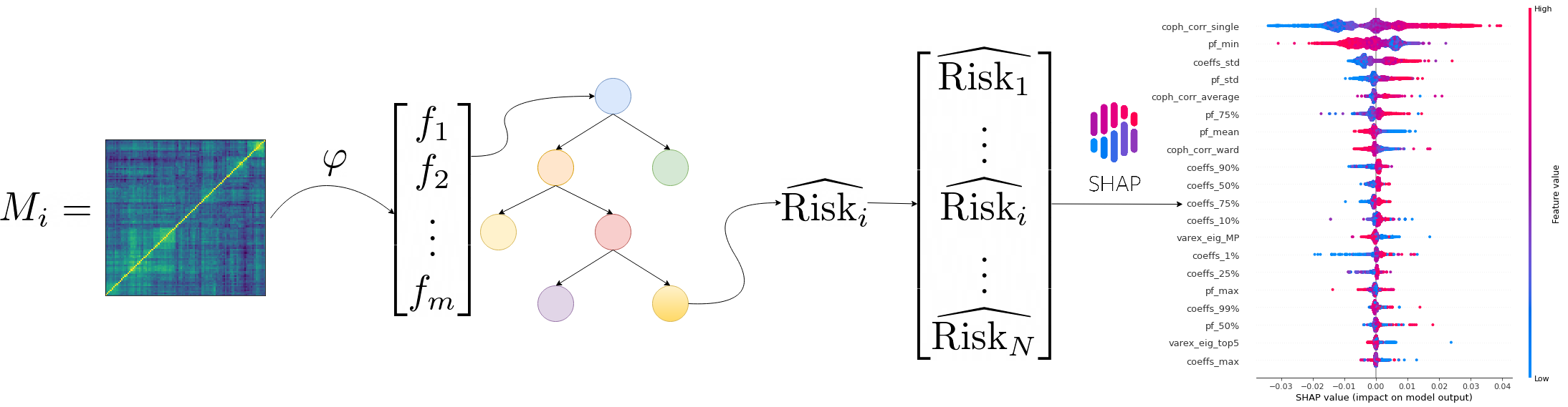
Extraction of features from a given correlation matrix
The step of extracting features from empirical correlation matrices was done in a previous blog post: Extraction of features from a given correlation matrix
TL;DR In order to describe as precisely as possible a given correlation matrix, we will extract a bunch of features from it. The features extracted and presented below are by no means exhaustive; It could be an ongoing research task to find other relevant features.
The features extracted from a given correlation matrix:
- Correlation coefficients distribution (mean, std, quantiles, min, max)
- Percentage of variance explained by the k-first eigenvalues, and by the eigenvalues above the Marchenko–Pastur law upper bound of its support
- First eigenvector summary statistics of its entries (mean, std, quantiles, min, max)
- Minimum Spanning Tree (MST) statistics based on shortest paths such as nodes’ closeness centrality, and average shortest path length
- Cophenetic correlation coefficient
- Condition number
These features aim at capturing several important properties of the correlation matrix:
- how strong the correlation is (e.g. correlation coefficients mean, first eigenvalue),
- how diverse the correlation can be (e.g. correlation coefficients std, first eigenvector std),
- how hierarchical the correlation structure is (e.g. cophenetic correlation)
- how complex and interconnected the system is (e.g. MST centrality quantiles and average shortest path length).
%matplotlib inline

import numpy as np
import pandas as pd
import scipy
from scipy.stats import rankdata
from numpy.polynomial.polynomial import polyfit
import shap
from sklearn import ensemble
from sklearn.inspection import permutation_importance
from sklearn.metrics import mean_squared_error
from sklearn.model_selection import train_test_split
from sklearn.model_selection import RandomizedSearchCV
import matplotlib.pyplot as plt
features = pd.read_hdf('empirical_features.h5')
features.shape
(12891, 36)
We have extracted 36 features for 12891 empirical correlation matrices.
Portfolio construction methods and risk metrics
This step has also been done in a previous blog post: Portfolio construction methods and risk metrics: in- and out-of-sample comparisons on simulated data.
TL;DR We simulate data using a 0-mean multivariate Gaussian and $t$-distribution with 3 degrees of freedom both parameterized with an empirical correlation matrix used as the correlation model.
From these distributions, we build two samples of $80 \times 500$ observations (approximately two years of daily returns for 80 stocks) each:
- an in-sample dataset used to estimate an empirical covariance matrix fed to a portfolio allocation method which returns weights,
- an out-of-sample dataset on which the weights previously computed are applied; risk metrics are then computed on the resulting portfolio returns.
As for risk metrics, we will compute:
- portfolio volatility,
- portfolio value at risk (VaR),
- portfolio expected shortfall (ES or CVaR),
- portfolio conditional drawdown-at-risk (CDaR).
We did such simulation and risks computation for each of the 12891 empirical correlation matrices used as a model for the data generating process (DGP).
We recover the results previously computed:
methods = ['uniform', 'HRP', 'inverse_variance', 'min_volatility',
           'max_return_min_volatility', 'max_diversification',
           'max_decorrelation',
           'equal_weighting', 'variance', 'standard_deviation',
           'expected_shortfall', 'conditional_drawdown_risk']

method_in_sample_risk = {method: [] for method in methods}
method_out_sample_risk = {method: [] for method in methods}

for method in methods:
    method_in_sample_risk[method] = np.load(
        f'risk_measures/{method}_risk_insample_student_3.npy')
    method_out_sample_risk[method] = np.load(
        f'risk_measures/{method}_risk_outsample_student_3.npy')
Now, we are ready to tackle Problems A and B.
Problem A: Predict outperformance of a portfolio allocation method over another one
Let’s first define our target variable for this problem: the difference in risk between methods 1 and 2.
def get_target_variable(method,
                        method_alt=None,
                        risk_metric='vol',
                        problem='perf_comparison'):
    risk_signs = [1, -1, -1, 1]

    if risk_metric == 'vol':
        id_r = 0
    elif risk_metric == 'VaR':
        id_r = 1
    elif risk_metric == 'CVaR':
        id_r = 2
    elif risk_metric == 'CDaR':
        id_r = 3
    else:
        print('Risk metric unknown.')
    sgn = risk_signs[id_r]

    if problem == 'perf_comparison' and method_alt is not None:
        y = (method_out_sample_risk[method][:, id_r] * sgn -
             method_out_sample_risk[method_alt][:, id_r] * sgn)
    elif problem == 'perf_decay':
        y = (method_out_sample_risk[method][:, id_r] -
             method_in_sample_risk[method][:, id_r])
    else:
        y = None
        print('Problem unknown.')

    return y
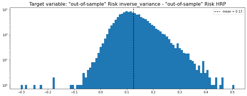
HRP vs. naive risk parity
method_1 = 'inverse_variance'
method_2 = 'HRP'

y = get_target_variable(method_1, method_2,
                        risk_metric='vol', problem='perf_comparison')
plt.figure(figsize=(14, 5))
plt.hist(y, bins=100, log=True)
plt.axvline(x=np.mean(y),
            color='k', linestyle='dashed',
            label='mean = {}'.format(round(np.mean(y), 2)))
plt.title(f'Target variable: "out-of-sample" Risk {method_1} - ' +
          f'"out-of-sample" Risk {method_2}',
          fontsize=16)
plt.legend()
plt.show()
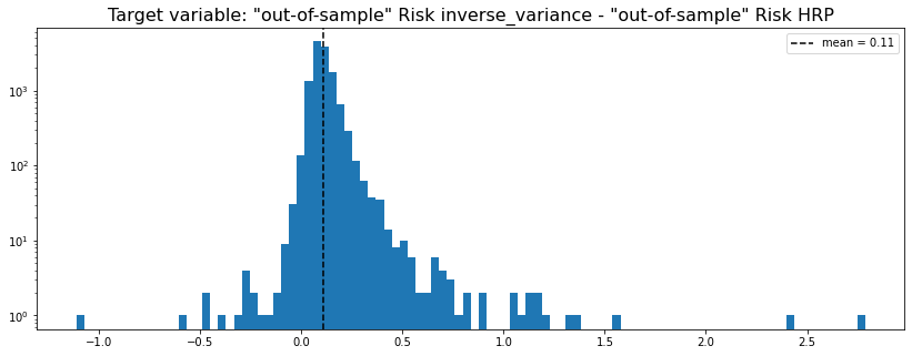
We can see that in average inverse_variance (naive risk parity) has a higher out-of-sample risk than the HRP (Hierarchical Risk Parity). We can also notice that the distribution is right-skewed; Arguments in favour of the HRP over this allocation method.
Can we predict when HRP beats naive risk parity? And why? Below some analytics to get a grasp at the answer:
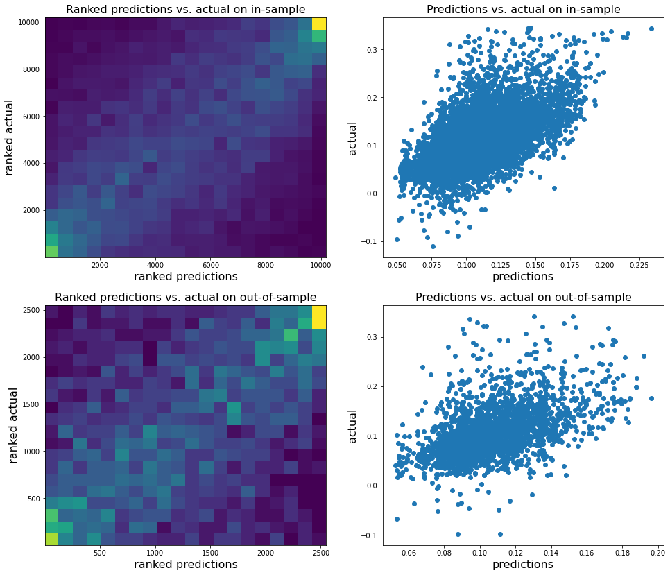
def display_pred_analytics(features, y, n_estimators=500):
z_scores = scipy.stats.zscore(y)
abs_z_scores = np.abs(z_scores)
filtered_entries = (abs_z_scores < 3)
y = y[filtered_entries]
features = features.iloc[filtered_entries, :]
X_train, X_test, y_train, y_test = train_test_split(
features, y, test_size=0.2, random_state=13)
params = {'n_estimators': n_estimators,
'max_depth': 5,
'min_samples_split': 5,
'learning_rate': 0.01,
'loss': 'ls'}
reg = ensemble.GradientBoostingRegressor(**params)
reg.fit(X_train, y_train)
mse = mean_squared_error(y_test, reg.predict(X_test))
print("The mean squared error (MSE) on test set: {:.4f}".format(mse))
test_score = np.zeros((params['n_estimators'],), dtype=np.float64)
for i, y_pred in enumerate(reg.staged_predict(X_test)):
test_score[i] = reg.loss_(y_test, y_pred)
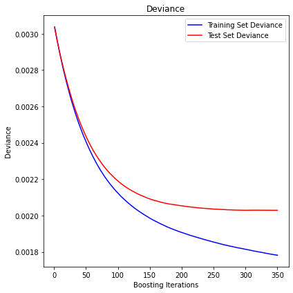
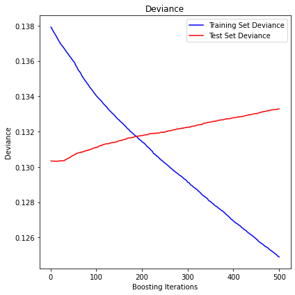
fig = plt.figure(figsize=(6, 6))
plt.subplot(1, 1, 1)
plt.title('Deviance')
plt.plot(np.arange(params['n_estimators']) + 1, reg.train_score_, 'b-',
label='Training Set Deviance')
plt.plot(np.arange(params['n_estimators']) + 1, test_score, 'r-',
label='Test Set Deviance')
plt.legend(loc='upper right')
plt.xlabel('Boosting Iterations')
plt.ylabel('Deviance')
fig.tight_layout()
plt.show()
print('R2 in-sample: {}'.format(round(reg.score(X_train, y_train), 2)))
print('R2 out-of-sample: {}'.format(round(reg.score(X_test, y_test), 2)))
print('Correlation predictions vs. actual in-sample: {}'.format(
round(np.corrcoef(reg.predict(X_train), y_train)[0, 1], 2)))
print('Correlation predictions vs. actual out-of-sample: {}'.format(
round(np.corrcoef(reg.predict(X_test), y_test)[0, 1], 2)))
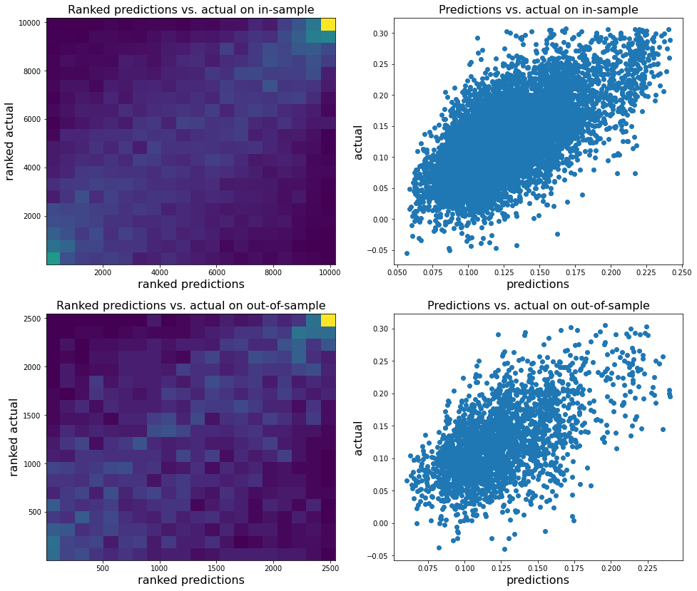
plt.figure(figsize=(16, 14))
plt.subplot(2, 2, 1)
plt.hist2d(rankdata(reg.predict(X_train)),
rankdata(y_train), bins=20)
plt.xlabel('ranked predictions', fontsize=16)
plt.ylabel('ranked actual', fontsize=16)
plt.title('Ranked predictions vs. actual on in-sample',
fontsize=16)
plt.subplot(2, 2, 2)
plt.scatter(reg.predict(X_train), y_train)
plt.xlabel('predictions', fontsize=16)
plt.ylabel('actual', fontsize=16)
plt.title('Predictions vs. actual on in-sample',
fontsize=16)
plt.subplot(2, 2, 3)
plt.hist2d(rankdata(reg.predict(X_test)),
rankdata(y_test), bins=20)
plt.xlabel('ranked predictions', fontsize=16)
plt.ylabel('ranked actual', fontsize=16)
plt.title('Ranked predictions vs. actual on out-of-sample',
fontsize=16)
plt.subplot(2, 2, 4)
plt.scatter(reg.predict(X_test), y_test)
plt.xlabel('predictions', fontsize=16)
plt.ylabel('actual', fontsize=16)
plt.title('Predictions vs. actual on out-of-sample',
fontsize=16)
plt.show()
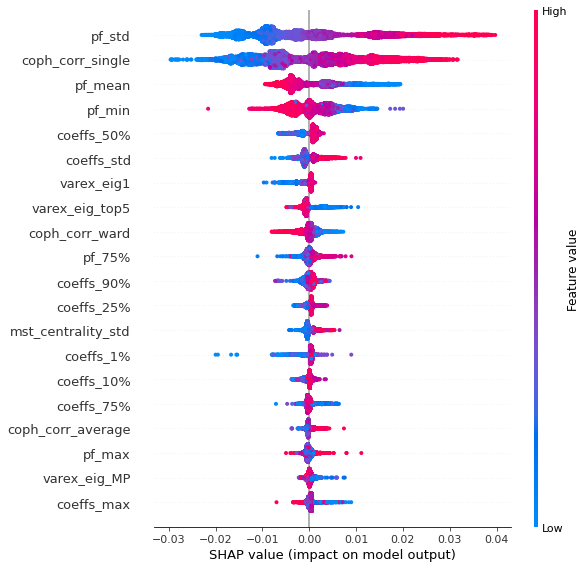
# Shapley values
explainer = shap.TreeExplainer(reg)
shap_values = explainer.shap_values(features)
shap.summary_plot(shap_values, features)
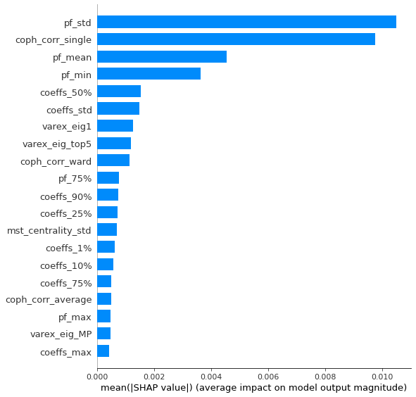
shap.summary_plot(shap_values, features, plot_type="bar")
sorted_idx = np.argsort(np.abs(shap_values).mean(axis=0))
feature_names = features.columns[sorted_idx][::-1][:5]
for col in feature_names:
# filter outliers on y and features[col]
df = pd.DataFrame(np.array([y, features[col]]),
index=['y', 'feature']).T
z_scores = scipy.stats.zscore(df)
abs_z_scores = np.abs(z_scores)
filtered_entries = (abs_z_scores < 3).all(axis=1)
clean_df = df[filtered_entries]
ranks = clean_df.rank() / len(clean_df)
plt.figure(figsize=(14, 5))
plt.subplot(1, 2, 1)
plt.hist2d(ranks['feature'], ranks['y'], bins=25)
plt.title(col)
plt.subplot(1, 2, 2)
b, m = polyfit(clean_df['feature'], clean_df['y'], 1)
plt.plot(clean_df['feature'], clean_df['y'], '.')
plt.plot(clean_df['feature'],
b + m * clean_df['feature'], '-')
plt.show()
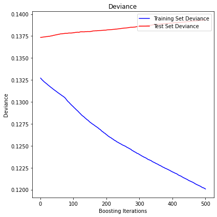
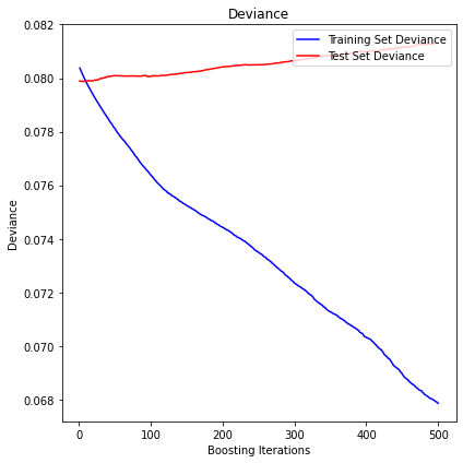
display_pred_analytics(features, y, n_estimators=350)
The mean squared error (MSE) on test set: 0.0020
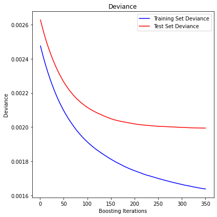
R2 in-sample: 0.34
R2 out-of-sample: 0.24
Correlation predictions vs. actual in-sample: 0.6
Correlation predictions vs. actual out-of-sample: 0.5
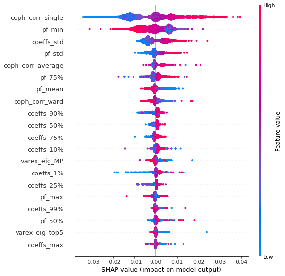
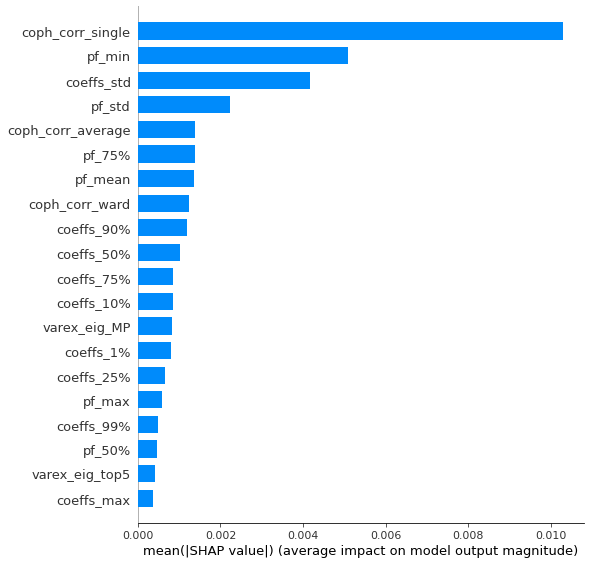
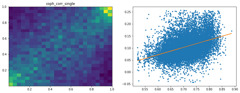
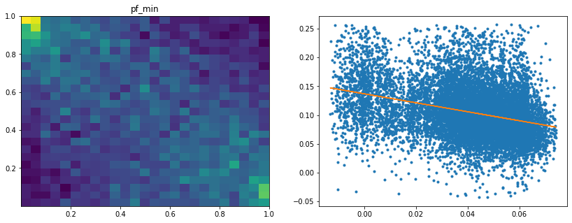
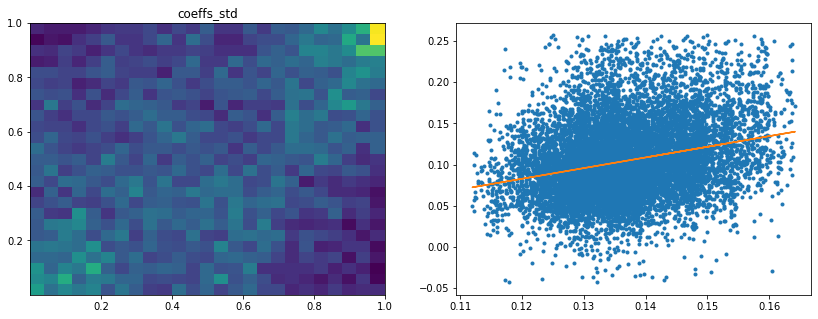
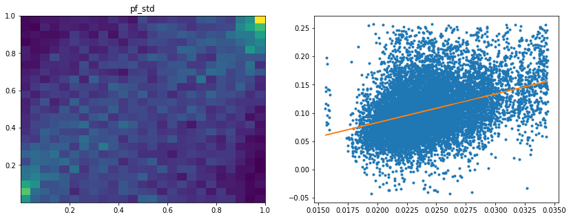
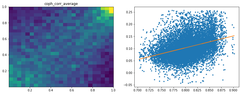
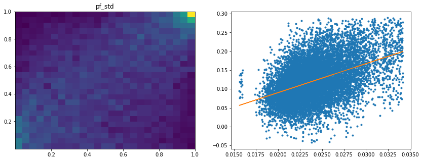
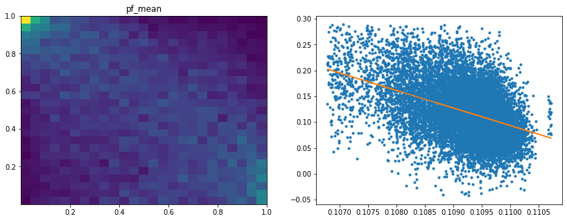
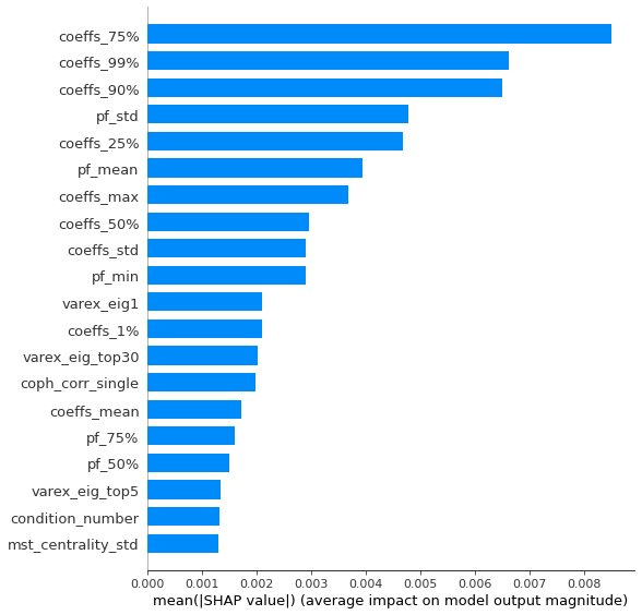
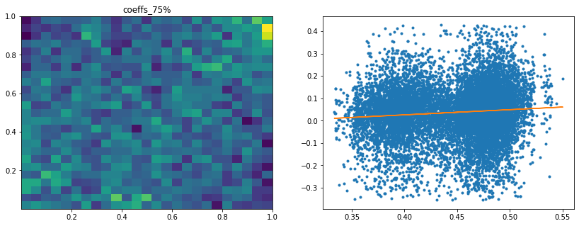
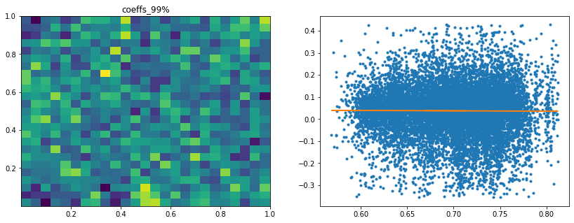
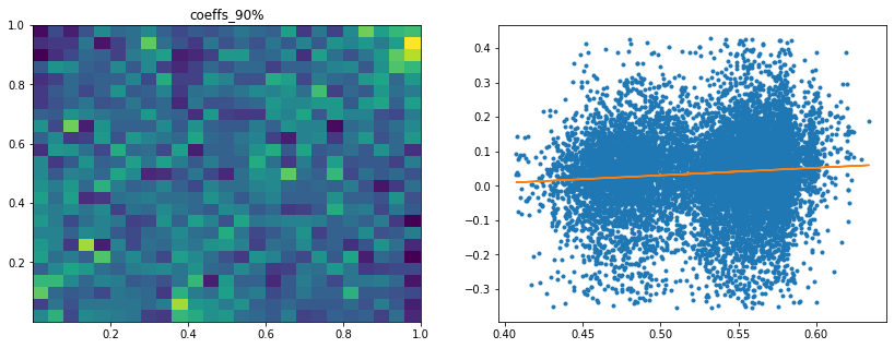
Analysis of the results: We observe that the most important features to determine whether Hierarchical Risk Parity will perform better (less risk) out-of-sample are the pf_std (or equivalently pf_mean as they are nearly perfectly correlated, cf. previous blog post) and the cophenetic correlation coefficient associated to the Single Linkage (used by the HRP algorithm). The Single Linkage cophenetic correlation coefficient is also strongly correlated to the pf_std (the standard deviation of the first eigenvector entries), especially when they both have high values.
High values for the cophenetic correlation coefficient are characteristic of a strong hierarchical structure. Thus, HRP outperforms naive risk parity when the underlying DGP has a strong hierarchical structure. When the correlation structure is quite flat, HRP performs similarly to the naive risk parity (or might underperform from time to time due to statistical noise).
We can repeat the same experience but using a different risk metric, namely the CVaR instead of the portfolio volatility:
method_1 = 'inverse_variance'
method_2 = 'HRP'

y = get_target_variable(method_1, method_2,
                        risk_metric='CVaR', problem='perf_comparison')
plt.figure(figsize=(14, 5))
plt.hist(y, bins=100, log=True)
plt.axvline(x=np.mean(y),
            color='k', linestyle='dashed',
            label='mean = {}'.format(round(np.mean(y), 2)))
plt.title(f'Target variable: "out-of-sample" Risk {method_1} - ' +
          f'"out-of-sample" Risk {method_2}',
          fontsize=16)
plt.legend()
plt.show()
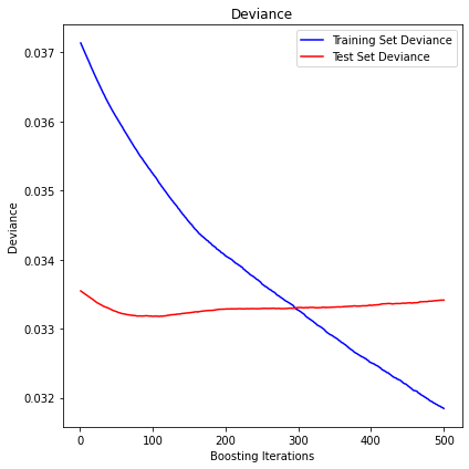
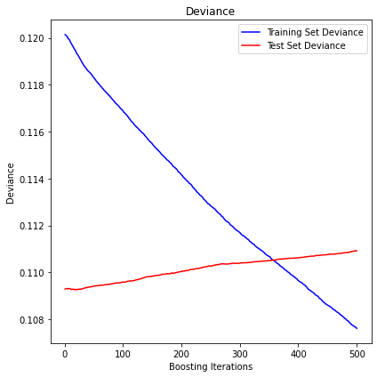
display_pred_analytics(features, y, n_estimators=350)
The mean squared error (MSE) on test set: 0.0020
R2 in-sample: 0.42
R2 out-of-sample: 0.33
Correlation predictions vs. actual in-sample: 0.65
Correlation predictions vs. actual out-of-sample: 0.58

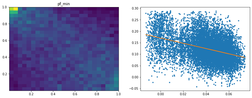
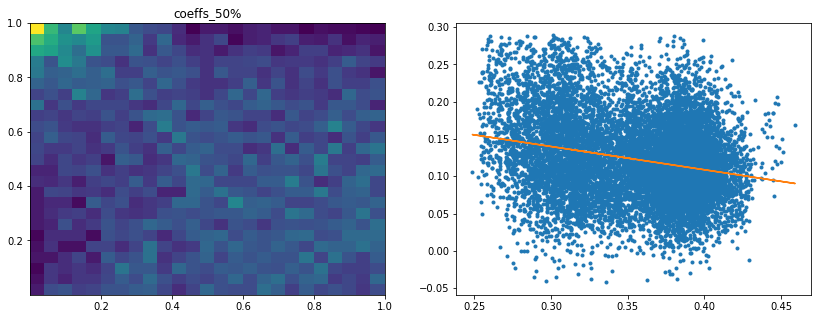
Analysis of the results: We notice similar results as in the previous experiment. It is rather easy to obtain a good predictive model of HRP relative outperformance based on the DGP correlation matrix features only. In average, for empirical correlation matrices, HRP outperforms its ‘flat’ counterpart the naive risk parity. Features driving HRP relative outperformance are again related to the first eigenvector coefficients dispersion (high pf_std impacts the output value higher, i.e. higher risk for naive risk parity than for HRP; low values of pf_min and high values of pf_max impact the output value higher, i.e. more relative outperformance of HRP when the first eigenvector entries are widely spread), and the cophenetic correlation coefficient of Single Linkage (the higher its values, the more effective HRP is compared to naive risk parity). When these features have high values, they hint at a stronger hierarchical correlation structure. Also, HRP does better when coeffs_50% and coeffs_std have high values. That is, when (median) correlation is high and when there is a big dispersion among the correlation matrix coefficients (hinting at strong clusters), then the naive risk parity tends to over-concentrate the risk, hence a relative outperformance from HRP.
In such cases, one should use HRP (preferably to naive risk parity).
Hierarchical 1/N vs. equally weighted
Similarly to the previous case where we compared the naive risk parity and ‘its’ hierarchical version the Hierarchical Risk Parity (actually, one out of its many possible hierarchical extension), we now compare the naive equally weighted allocation uniform to ‘its’ hierarchical version the Hierarchical 1/N equal_weighting:
method_1 = 'uniform' # equally weighted
method_2 = 'equal_weighting' # Hierarchical 1/N

y = get_target_variable(method_1, method_2,
                        risk_metric='vol', problem='perf_comparison')
plt.figure(figsize=(14, 5))
plt.hist(y, bins=100, log=True)
plt.axvline(x=np.mean(y),
            color='k', linestyle='dashed',
            label='mean = {}'.format(round(np.mean(y), 2)))
plt.title(f'Target variable: "out-of-sample" Risk {method_1} - ' +
          f'"out-of-sample" Risk {method_2}',
          fontsize=16)
plt.legend()
plt.show()
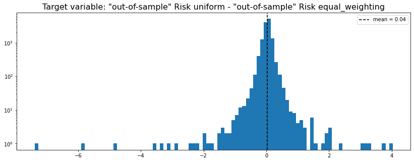
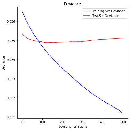
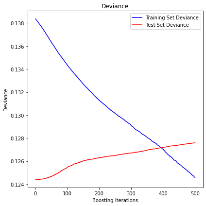
display_pred_analytics(features, y, n_estimators=350)
The mean squared error (MSE) on test set: 0.0160
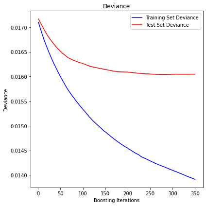
R2 in-sample: 0.19
R2 out-of-sample: 0.07
Correlation predictions vs. actual in-sample: 0.49
Correlation predictions vs. actual out-of-sample: 0.26
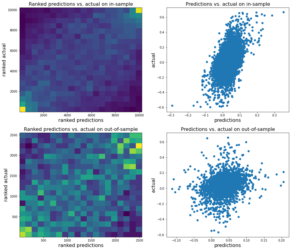
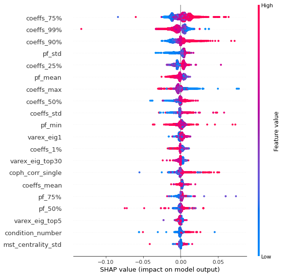
Analysis of the results: In average, the Hierarchical 1/N outperforms the equally weighted allocation method. In this case, we can find a smaller but decent predictability of the outperformance based on the DGP correlation matrix features only. The important features in this case are:
- the correlation matrix coefficients quantiles: When q=75%, 90%, 25%, 50% have high values, Hierarchical 1/N outperforms;
- the correlation matrix coefficients dispersion: With high values, Hierarchical 1/N tends to outperform;
- with low values of dispersion in the first eigenvector coefficients, equally weighted tends to outperform the Hierarchical 1/N;
- with low values of q=99% and coeffs_max for correlation matrix coefficients, equally weighted tends to outperform.
This feature importance analysis hints at the presence or no of a strong clustering structure.
For Hierarchical 1/N to outperform, one needs strong correlations yet high dispersion in the coefficients, i.e. neatly delimited clusters with strong intra-correlation and low inter-correlation between the clusters.
However, if there are a couple of extremely correlated assets (q=99% or coeffs_max high), chances are that the Hierarchical 1/N will over-allocate to them (check the method definition to convince you of that) as they will constitute a well-separated small cluster appearing early on and being merge toward the end to the rest of the dendrogram: Thus, they will get too much allocation. In such cases, prefer the equally weighted method. The Hierarchical 1/N works best when there are homogeneous clusters and a well-balanced dendrogram. Not necessarily the case with typical correlation matrices of stocks…
If there is no strong clustering structure, then Hierarchical 1/N does not outperform its ‘flat’ counterpart as evidenced by the fact that with low values of dispersion in the first eigenvector coefficients, the equally weighted method tends to outperform. More precisely, this low dispersion means that the entries in the first eigenvector have roughly the same value, i.e. assets are all exposed roughly equally to the first factor which explains the most variance, hence no clusters.
To back up further this analysis, one should re-run this experiment with more features such as q=99% - q=90%, varex_eig_top5 - varex_eig_1, and other features aiming at quantifying the clustering strength.
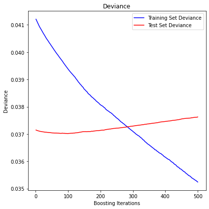
Problem B: Predict decay in performance from in-sample to out-of-sample
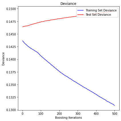
Can we predict the out-of-sample performance decay based solely on the DGP correlation matrix features?
risk_signs = [1, -1, -1, 1]
id_r = 0
sgn = risk_signs[id_r]

for method in methods:
    print(method)

    y = (method_out_sample_risk[method][:, id_r] * sgn -
         method_in_sample_risk[method][:, id_r] * sgn)

    features = pd.read_hdf('empirical_features.h5')

    z_scores = scipy.stats.zscore(y)
    abs_z_scores = np.abs(z_scores)
    filtered_entries = (abs_z_scores < 3)
    y = y[filtered_entries]
    features = features.iloc[filtered_entries, :]

    X_train, X_test, y_train, y_test = train_test_split(
        features, y, test_size=0.2, random_state=13)

    params = {'n_estimators': 500,
              'max_depth': 5,
              'min_samples_split': 5,
              'learning_rate': 0.01,
              'loss': 'ls'}

    reg = ensemble.GradientBoostingRegressor(**params)
    reg.fit(X_train, y_train)

    mse = mean_squared_error(y_test, reg.predict(X_test))
    print("The mean squared error (MSE) on test set: {:.4f}".format(mse))

    test_score = np.zeros((params['n_estimators'],), dtype=np.float64)
    for i, y_pred in enumerate(reg.staged_predict(X_test)):
        test_score[i] = reg.loss_(y_test, y_pred)

    fig = plt.figure(figsize=(6, 6))
    plt.subplot(1, 1, 1)
    plt.title('Deviance')
    plt.plot(np.arange(params['n_estimators']) + 1, reg.train_score_, 'b-',
             label='Training Set Deviance')
    plt.plot(np.arange(params['n_estimators']) + 1, test_score, 'r-',
             label='Test Set Deviance')
    plt.legend(loc='upper right')
    plt.xlabel('Boosting Iterations')
    plt.ylabel('Deviance')
    fig.tight_layout()
    plt.show()

    print('R2 in-sample: {}'.format(round(reg.score(X_train, y_train), 2)))
    print('R2 out-of-sample: {}'.format(round(reg.score(X_test, y_test), 2)))
    print('Correlation predictions vs. actual in-sample: {}'.format(
        round(np.corrcoef(reg.predict(X_train), y_train)[0, 1], 2)))
    print('Correlation predictions vs. actual out-of-sample: {}\n'.format(
        round(np.corrcoef(reg.predict(X_test), y_test)[0, 1], 2)))
uniform
The mean squared error (MSE) on test set: 0.3029
R2 in-sample: 0.16
R2 out-of-sample: -0.03
Correlation predictions vs. actual in-sample: 0.55
Correlation predictions vs. actual out-of-sample: -0.03


HRP
The mean squared error (MSE) on test set: 0.0967
R2 in-sample: 0.1
R2 out-of-sample: -0.02
Correlation predictions vs. actual in-sample: 0.44
Correlation predictions vs. actual out-of-sample: -0.03


inverse_variance
The mean squared error (MSE) on test set: 0.1393
R2 in-sample: 0.1
R2 out-of-sample: -0.01
Correlation predictions vs. actual in-sample: 0.44
Correlation predictions vs. actual out-of-sample: -0.01


min_volatility
The mean squared error (MSE) on test set: 0.0334
R2 in-sample: 0.14
R2 out-of-sample: 0.0
Correlation predictions vs. actual in-sample: 0.48
Correlation predictions vs. actual out-of-sample: 0.1


max_return_min_volatility
The mean squared error (MSE) on test set: 0.0351
R2 in-sample: 0.15
R2 out-of-sample: 0.01
Correlation predictions vs. actual in-sample: 0.49
Correlation predictions vs. actual out-of-sample: 0.1


max_diversification
The mean squared error (MSE) on test set: 0.0376
R2 in-sample: 0.15
R2 out-of-sample: -0.01
Correlation predictions vs. actual in-sample: 0.5
Correlation predictions vs. actual out-of-sample: 0.04


max_decorrelation
The mean squared error (MSE) on test set: 0.0813
R2 in-sample: 0.16
R2 out-of-sample: -0.02
Correlation predictions vs. actual in-sample: 0.5
Correlation predictions vs. actual out-of-sample: 0.03


equal_weighting
The mean squared error (MSE) on test set: 0.1109
R2 in-sample: 0.1
R2 out-of-sample: -0.02
Correlation predictions vs. actual in-sample: 0.47
Correlation predictions vs. actual out-of-sample: 0.0


variance
The mean squared error (MSE) on test set: 0.1276
R2 in-sample: 0.1
R2 out-of-sample: -0.03
Correlation predictions vs. actual in-sample: 0.46
Correlation predictions vs. actual out-of-sample: -0.03


standard_deviation
The mean squared error (MSE) on test set: 0.1495
R2 in-sample: 0.09
R2 out-of-sample: -0.02
Correlation predictions vs. actual in-sample: 0.43
Correlation predictions vs. actual out-of-sample: -0.03


expected_shortfall
The mean squared error (MSE) on test set: 0.1582

R2 in-sample: 0.1
R2 out-of-sample: -0.02
Correlation predictions vs. actual in-sample: 0.48
Correlation predictions vs. actual out-of-sample: -0.0


conditional_drawdown_risk
The mean squared error (MSE) on test set: 0.1333
R2 in-sample: 0.09
R2 out-of-sample: -0.02
Correlation predictions vs. actual in-sample: 0.44
Correlation predictions vs. actual out-of-sample: -0.03
Analysis of the results: No predictability found.
Conclusion: In this blog post, we set two goals:
-
Can we predict the relative outperformance of a method over the others from the correlation matrix features only? If so, which features are the most important?
-
Can we predict for a given method its decrease in performance between the in-sample and out-of-sample from the correlation matrix features only? If so, which features are the most important?
Solving these questions would give some guidance on the choice of a portfolio allocation method: It will rely on the current correlation regime and its features (or the one we forecast will prevail in the future).
We empirically found evidence that predicting outperformance of a portfolio allocation method over another one based on the correlation matrix features is a feasible task. Furthermore, the features importance attribution hints at features which make intuitive sense for this prediction task given the definition and construction of the portfolio methods. All this suggests that this is a promising research avenue.
On the other hand, we found no predictability for the performance decay between the in- and out-of-sample. This shall be investigated further.