Can we predict a market regime from correlation matrix features?
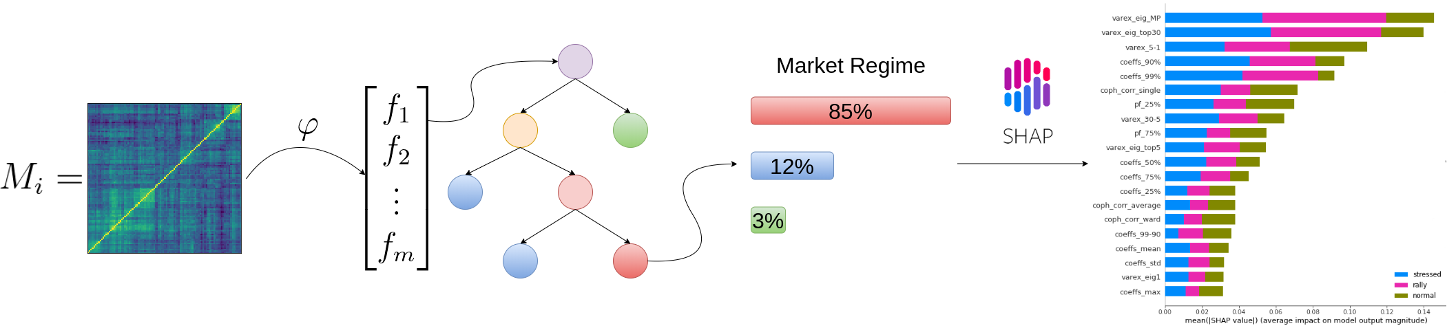
Can we predict a market regime from correlation matrix features?
In a previous blog, we estimated correlation matrices associated to three different market regimes: stressed, normal, rally. We defined the market regimes somewhat arbitrarily, based on the Sharpe ratio of an equi-weighted portfolio of stocks. If the Sharpe ratio is below -0.5, stressed market regime; above 2, rally market regimes; otherwise, normal. Details there: S&P 500 Sharpe vs. Correlation Matrices - Building a dataset for generating stressed/rally/normal scenarios.
In this blog, we follow-up on the ideas exposed in:
We will:
- Study the distribution of the correlation matrix features for the different regimes,
- Try to answer whether we can determine the market regime based on the correlation matrix features only.
For 2., we will cast this question into a classification problem. We do not expect perfect classification since the definition of the classes (stressed, normal, rally) is somewhat arbitrary and rather clumsy: Why would an equi-weighted long-only Sharpe 1.99 portfolio associated to a normal market regime whereas a Sharpe 2.01 portfolio considered benefitting from a market rally?
TL;DR From the correlation matrix features only, we can determine rather easily which market regime is happening.
This result is interesting: Despite discarding the expected returns and volatility information, we are able to find a good mapping between the correlation matrix features and the market regime. It would be worthwhile to test it against other, and maybe more sophisticated, definitions of market regime; And also on other markets.
We find that
- feat1 = ‘varex_eig_MP’
- feat2 = ‘coph_corr_single’
are the most important (low correlation pair of) features to be able to distinguish between the 3 classes ‘rally’, ‘stressed’, ‘normal’.
It’s even possible to fit a decent model with only those two.
%matplotlib inline

from multiprocessing import Pool
import tqdm
import numpy as np
import pandas as pd
from scipy.cluster import hierarchy
from scipy.cluster.hierarchy import cophenet
from sklearn.model_selection import train_test_split
from sklearn.ensemble import RandomForestClassifier
from sklearn.metrics import confusion_matrix
import fastcluster
import networkx as nx
import shap
import matplotlib.pyplot as plt
import warnings
warnings.filterwarnings("ignore")
def compute_mst_stats(corr):
    dist = (1 - corr) / 2
    G = nx.from_numpy_matrix(dist)
    mst = nx.minimum_spanning_tree(G)

    features = pd.Series()
    features['mst_avg_shortest'] = nx.average_shortest_path_length(mst)


    closeness_centrality = (pd
                            .Series(list(nx
                                         .closeness_centrality(mst)
                                         .values()))
                            .describe())
    for stat in closeness_centrality.index[1:]:
        features[f'mst_centrality_{stat}'] = closeness_centrality[stat]

    return features

def compute_intravar_clusters(model_corr, Z, nb_clusters=5):
    clustering_inds = hierarchy.fcluster(Z, nb_clusters,
                                         criterion='maxclust')
    clusters = {i: [] for i in range(min(clustering_inds),
                                     max(clustering_inds) + 1)}
    for i, v in enumerate(clustering_inds):
        clusters[v].append(i)

    total_var = 0
    for cluster in clusters:
        sub_corr = model_corr[clusters[cluster], :][:, clusters[cluster]]
        sa, sb = np.triu_indices(sub_corr.shape[0], k=1)
        mean_corr = sub_corr[sa, sb].mean()
        cluster_var = sum(
            [(sub_corr[i, j] - mean_corr)**2 for i in range(len(sub_corr))
             for j in range(i + 1, len(sub_corr))])
        total_var += cluster_var

    return total_var

def compute_features_from_correl(model_corr):
    n = len(model_corr)
    a, b = np.triu_indices(n, k=1)

    features = pd.Series()
    coefficients = model_corr[a, b].flatten()

    coeffs = pd.Series(coefficients)
    coeffs_stats = coeffs.describe()
    for stat in coeffs_stats.index[1:]:
        features[f'coeffs_{stat}'] = coeffs_stats[stat]
    features['coeffs_1%'] = coeffs.quantile(q=0.01)
    features['coeffs_99%'] = coeffs.quantile(q=0.99)
    features['coeffs_10%'] = coeffs.quantile(q=0.1)
    features['coeffs_90%'] = coeffs.quantile(q=0.9)
    features['coeffs_99-90'] = features['coeffs_99%'] - features['coeffs_90%']
    features['coeffs_10-1'] = features['coeffs_10%'] - features['coeffs_1%']


    # eigenvals
    eigenvals, eigenvecs = np.linalg.eig(model_corr)
    permutation = np.argsort(eigenvals)[::-1]
    eigenvals = eigenvals[permutation]
    eigenvecs = eigenvecs[:, permutation]

    pf_vector = eigenvecs[:, np.argmax(eigenvals)]
    if len(pf_vector[pf_vector < 0]) > len(pf_vector[pf_vector > 0]):
        pf_vector = -pf_vector

    features['varex_eig1'] = float(eigenvals[0] / sum(eigenvals))
    features['varex_eig_top5'] = (float(sum(eigenvals[:5])) /
        float(sum(eigenvals)))
    features['varex_eig_top30'] = (float(sum(eigenvals[:30])) /
        float(sum(eigenvals)))
    features['varex_5-1'] = (features['varex_eig_top5'] -
        features['varex_eig1'])
    features['varex_30-5'] = (features['varex_eig_top30'] -
        features['varex_eig_top5'])
    # Marcenko-Pastur (RMT)
    T, N = 252, n
    MP_cutoff = (1 + np.sqrt(N / T))**2
    # variance explained by eigenvals outside of the MP distribution
    features['varex_eig_MP'] = (
        float(sum([e for e in eigenvals if e > MP_cutoff])) /
        float(sum(eigenvals)))

    # determinant
    features['determinant'] = np.prod(eigenvals)

    # condition number
    features['condition_number'] = abs(eigenvals[0]) / abs(eigenvals[-1])


    # stats of the first eigenvector entries
    pf_stats = pd.Series(pf_vector).describe()
    for stat in pf_stats.index[1:]:
        features[f'pf_{stat}'] = float(pf_stats[stat])


    # stats on the MST
    features = pd.concat([features, compute_mst_stats(model_corr)],
                         axis=0)

    # stats on the linkage
    dist = np.sqrt(2 * (1 - model_corr))
    for algo in ['ward', 'single', 'complete', 'average']:
        Z = fastcluster.linkage(dist[a, b], method=algo)
        features[f'coph_corr_{algo}'] = cophenet(Z, dist[a, b])[0]

    # stats on the clusters
    Z = fastcluster.linkage(dist[a, b], method='ward')
    features['cl_intravar_5'] = compute_intravar_clusters(
        model_corr, Z, nb_clusters=5)
    features['cl_intravar_10'] = compute_intravar_clusters(
        model_corr, Z, nb_clusters=10)
    features['cl_intravar_25'] = compute_intravar_clusters(
        model_corr, Z, nb_clusters=25)
    features['cl_intravar_5-10'] = (
        features['cl_intravar_5'] - features['cl_intravar_10'])
    features['cl_intravar_10-25'] = (
        features['cl_intravar_10'] - features['cl_intravar_25'])

    return features.sort_index()
def compute_dataset_features(mats):
    all_features = []
    for i in range(mats.shape[0]):
        model_corr = mats[i, :, :]

        features = compute_features_from_correl(model_corr)

        if features is not None:
            all_features.append(features)

    return pd.concat(all_features, axis=1).T
def compute_dataset_features__par(mats):
    p = Pool(3)
    all_features = p.imap(compute_features_from_correl,
                          tqdm.tqdm([mats[i, :, :]
                                     for i in range(mats.shape[0])]))
    p.close()
    p.join()

    return pd.concat(all_features, axis=1).T
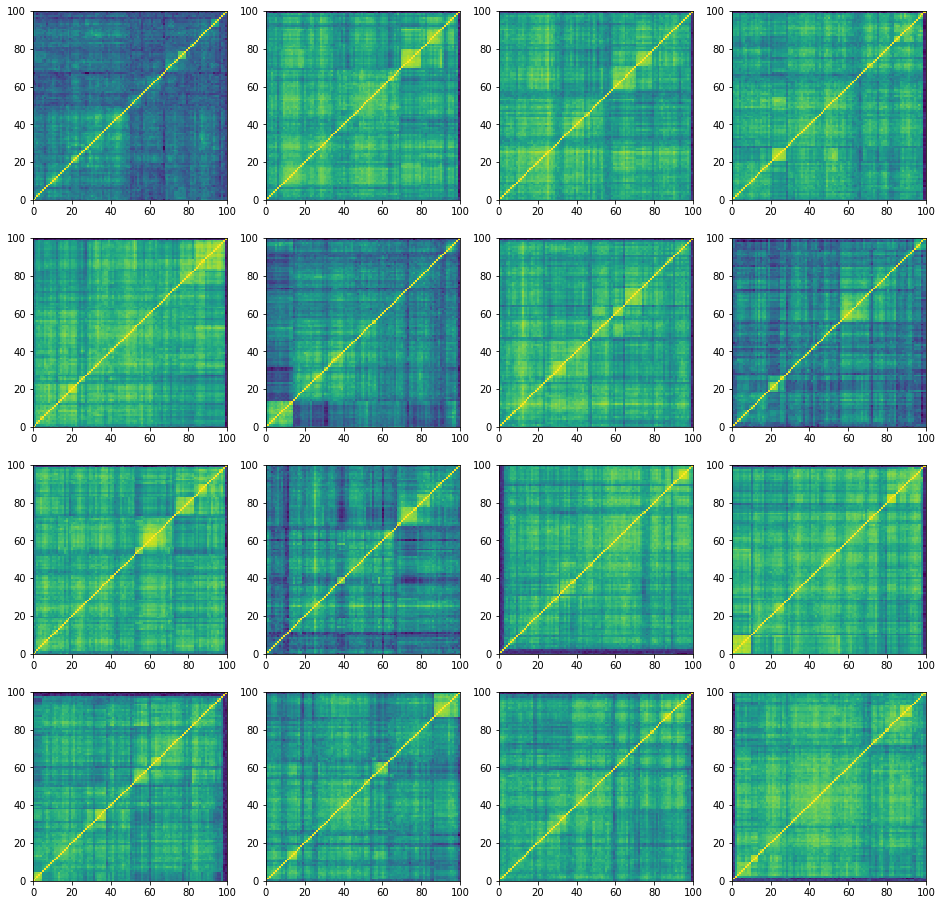
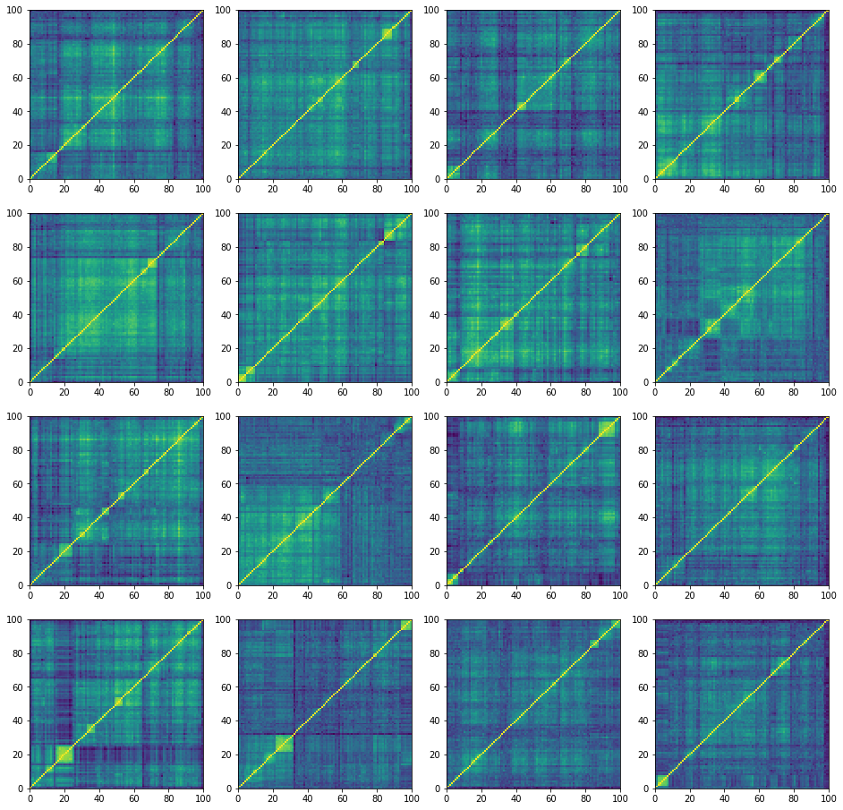
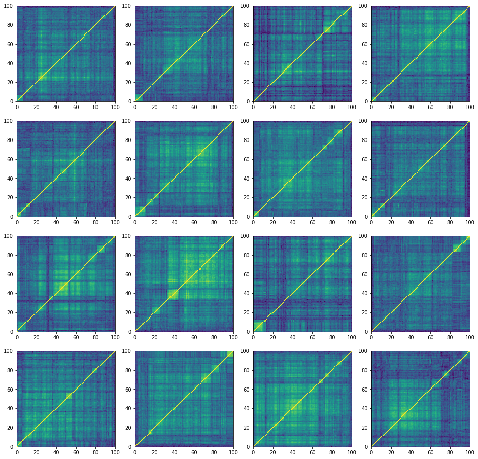
regimes = ['stressed', 'normal', 'rally']
regime_features = {}
for regime in regimes:
    corr_matrices = np.load(f'{regime}_matrices.npy')

    plt.figure(figsize=(16, 16))
    for i in range(16):
        corr = corr_matrices[i, :, :]
        plt.subplot(4, 4, i + 1)
        plt.pcolormesh(corr)
    plt.show()

    corr_features = compute_dataset_features__par(corr_matrices)

    regime_features[regime] = corr_features.astype(float)
‘stressed’ correlation matrices:
100%|██████████| 27000/27000 [25:34<00:00, 17.59it/s]
‘normal’ correlation matrices:
100%|██████████| 27000/27000 [24:41<00:00, 18.23it/s]
‘rally’ correlation matrices:
100%|██████████| 27000/27000 [24:01<00:00, 18.72it/s]
We save the features for future use.
for regime in regimes:
    regime_features[regime].to_hdf(
        f'regime_{regime}_features.h5', key='features')
regimes = ['stressed', 'normal', 'rally']
regime_features = {}
for regime in regimes:
    regime_features[regime] = pd.read_hdf(f'regime_{regime}_features.h5')
Some exploratory data analysis on the features. Plotting their distribution:
colors = ['r', 'b', 'g']
plt.figure(figsize=(16, 40))
for idx, col in enumerate(regime_features['stressed'].columns):
    plt.subplot(12, 4, idx + 1)
    for ic, regime in enumerate(['stressed', 'normal', 'rally']):
        qlow = regime_features[regime][col].quantile(0.01)
        qhigh = regime_features[regime][col].quantile(0.99)
        plt.hist(regime_features[regime][col]
                 .clip(lower=qlow, upper=qhigh)
                 .replace(qlow, np.nan)
                 .replace(qhigh, np.nan),
                 bins=100, log=False, color=colors[ic], alpha=0.5)
        plt.axvline(x=regime_features[regime][col].mean(), color=colors[ic],
                    linestyle='dashed', linewidth=2)
    plt.title(col)
    plt.legend(regimes)
plt.show()
We can observe that for many features, the stressed market regime has a very different distribution shape. For example, the variance explained by a few top principal components is much higher for the stressed regime than for the normal and rally ones. In stressed regime, absolute average correlation is higher (first eigenvalue), but also the correlation between and within industries. It means, in stressed regime, the hierarchy of correlations and the associated clusters are not well defined. This can be seen from the distributions of the cophenetic correlation coefficients: They are localized at a lower value in the case of the stressed regime than they are for the rally and normal cases (which have very similar distributions). It can also be observed from the distribution of varex_30-5 (the difference in variance explained by 30 factors and 5 factors): in a stressed regime, 30 factors do not explain much more variance than 5 factors, whereas in a rally (and to some extent in a normal regime) 30 factors explain the data much better than the first 5 principal components can.
We can also remark that the condition number is high (and the determinant is close to 0) in the stressed regime: Allocation methods based on a naive inverse of the covariance (correlation) matrix will likely fail. This is also the case to some extent for the normal regime, whereas the correlation matrices associated to the rally regime are well-conditioned (easier to invert). However, in a rally regime, proper diversification is less critical than during a stressed regime: Diversification may fail when it is the most needed.
Based on these quick observations, we can hope that a good classifier (stressed, normal, rally) can be easily obtained. The stressed regime class should be separated very easily since the associated features distributions are localized well apart from the normal and rally features distributions. For the latter, their support is strongly overlapping (cf. Bayes error rate), and sometimes they share the same modes, i.e. it will be harder for the classifier to put them apart. The ‘variance explained top 5, MP, 30’ features should be the ones helping for these ‘rally’ and ‘normal’ classes.
To summarize so far:
-
We did a quick features analysis pre-classification stage;
-
Main insights gained: the classification problem shouldn’t be hard, we can guess that
  - variance explained,
  - cophenetic correlation coefficient,
  - mean correlation,
  - and to some extent condition number, first eigenvector
should be helpful features for the classifier, whereas
  - clusters intra-variance,
  - minimum spanning tree centrality stats
should be close to useless for the classifier.
Can we build a good classifier?
Let’s do a basic random forest using Scikit-Learn, without any (fine-)tuning.
for regime in regimes:
    regime_features[regime]['target'] = regime

data = pd.concat([regime_features[regime] for regime in regimes], axis=0)
data = data.reset_index(drop=True)
X_train, X_test, y_train, y_test = train_test_split(
    data.loc[:, data.columns != 'target'], data['target'],
    test_size=0.2, random_state=13)
clf = RandomForestClassifier(random_state=42)
clf.fit(X_train, y_train)

print('Accuracy on train set:', clf.score(X_train, y_train))
print('Accuracy on test set:', clf.score(X_test, y_test))
Accuracy on train set: 1.0
Accuracy on test set: 0.802944035550618
labels = ['stressed', 'normal', 'rally']
confusion_mat = confusion_matrix(
    y_test, clf.predict(X_test), labels=labels)
def plot_confusion_matrix(cm,
                          target_names,
                          title='Confusion matrix',
                          cmap=None,
                          normalize=True):
    import itertools

    accuracy = np.trace(cm) / np.sum(cm).astype('float')

    if cmap is None:
        cmap = plt.get_cmap('Blues')

    plt.figure(figsize=(8, 6))
    plt.imshow(cm, interpolation='nearest', cmap=cmap)
    plt.title(title)
    plt.colorbar()

    if target_names is not None:
        tick_marks = np.arange(len(target_names))
        plt.xticks(tick_marks, target_names, rotation=45)
        plt.yticks(tick_marks, target_names)

    if normalize:
        cm = cm.astype('float') / cm.sum(axis=1)[:, np.newaxis]


    thresh = cm.max() / 1.5 if normalize else cm.max() / 2
    for i, j in itertools.product(range(cm.shape[0]), range(cm.shape[1])):
        if normalize:
            plt.text(j, i, "{:0.2f}".format(cm[i, j]),
                     horizontalalignment="center",
                     color="white" if cm[i, j] > thresh else "black")
        else:
            plt.text(j, i, "{:,}".format(cm[i, j]),
                     horizontalalignment="center",
                     color="white" if cm[i, j] > thresh else "black")

    plt.tight_layout()
    plt.ylabel('True label')
    plt.xlabel('Predicted label\naccuracy={:0.2f}'.format(accuracy))
    plt.show()
plot_confusion_matrix(confusion_mat, labels)
The confusion matrix essentially gives frequencies of correct and wrong answers. However, the model could be correct but with a low confidence.
Let’s display the average confidence of the model on the test set, conditioned on a given predicted class (but not conditioned on being correct).
proba = clf.predict_proba(X_test)

labels = ['normal', 'rally', 'stressed']
plt.figure(figsize=(18, 5))
for id_class, cls in enumerate(labels):
    plt.subplot(1, 3, id_class + 1)
    x = proba[proba.argmax(axis=1) == id_class]
    print(f'Number of {cls} data-points:\t {x.shape[0]}')
    plt.bar(labels, x.mean(axis=0),
        color=['blue', 'green', 'red'])
    plt.title(
        f'Average classifier confidence given class = {cls}')
plt.show()
Number of normal data-points:	 4215
Number of rally data-points:	 6213
Number of stressed data-points:	 5772
We can observe that when the model predicts the ‘stressed’ class, in average it is more confident than when predicting another class. Also, there is not much doubt possible between the ‘rally’ class and the ‘stressed’ class; most of the model uncertainty is between ‘rally’ and ‘normal’, and to some extent also between ‘stressed’ and ‘normal’.
We also check the average confidence of the model on the test set, conditioned this time both on a given predicted class and being correct:
proba = clf.predict_proba(X_test)

labels = ['normal', 'rally', 'stressed']
str2int = {s: idc for idc, s in enumerate(labels)}
plt.figure(figsize=(18, 5))
for id_class, cls in enumerate(labels):
    plt.subplot(1, 3, id_class + 1)
    majority_class = proba.argmax(axis=1) == id_class
    correct_class = (proba.argmax(axis=1) ==
                     [str2int[y] for y in y_test])
    x = proba[majority_class & correct_class]
    print(f'Number of {cls} data-points:\t {x.shape[0]}')
    plt.bar(labels, x.mean(axis=0),
        color=['blue', 'green', 'red'])
    plt.title(
        f'Average confidence given class = {cls} & correct')
plt.show()
Number of normal data-points:	 3372
Number of rally data-points:	 4853
Number of stressed data-points:	 4984
As expected, the stressed regime is the easiest to classify. Most of the confusion is on the ‘normal’ class. This is not unexpected since
-
it is the usual market state that can transition toward a more extreme one (rally or stressed),
-
the classes are not super well-defined from the start, and it could be that some predictions deemed as errors are actually correct.
For the latter reason, we also define a subet of the data which corresponds to correlation matrices where the classifier has high confidence (above 90%), i.e. data-points which are well inside the decision boundaries.
We will check that results/insights found on the whole training and testing datasets are also stable on their corresponding high confidence subsets. If it is not the case, it could mean that results/insights are essentially driven by data-points on the decision boundaries (close points can have a different class; the confidence of the model in those regions is usually lower) whose respective ground-truth class is not certain to be correct.
def get_high_confidence(X, y):
    pred = clf.predict_proba(X)
    high_confidence_features = X.iloc[pred.max(axis=1) > 0.90]
    high_confidence_labels = y.iloc[pred.max(axis=1) > 0.90]

    return high_confidence_features, high_confidence_labels
features_train, labels_train = get_high_confidence(X_train, y_train)
labels_train.value_counts()
stressed    15943
rally       11564
normal       7848
Name: target, dtype: int64
features_test, labels_test = get_high_confidence(X_test, y_test)
labels_test.value_counts()
stressed    2739
normal      1524
rally        928
Name: target, dtype: int64
clf = RandomForestClassifier(random_state=42)
clf.fit(X_train, y_train)

print('Accuracy on test set:', round(clf.score(X_test, y_test), 2))
print('Accuracy on test set when model has high confidence:',
      round(clf.score(features_test, labels_test), 2))
Accuracy on test set: 0.8
Accuracy on test set when model has high confidence: 0.99
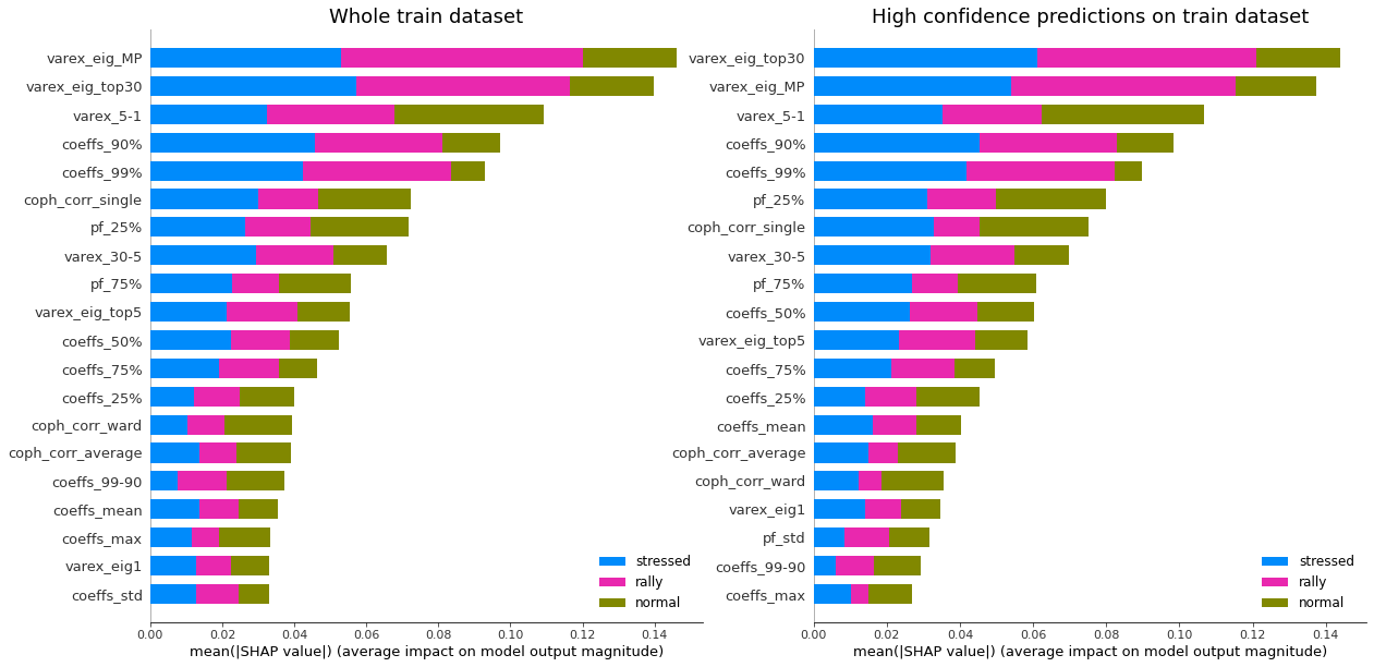
What are the relevant features for this model?
def display_shap_importance(X, X_high_confidence, sample_type='train'):
    height = 10
    width = 20
    plt.figure(figsize=(height, width))
    plt.subplot(1, 2, 1)
    # shap on the whole dataset
    explainer = shap.TreeExplainer(clf)
    shap_values = explainer.shap_values(X, approximate=True)
    shap.summary_plot(shap_values, X,
                      plot_type="bar",
                      class_names=['normal', 'rally', 'stressed'],
                      plot_size=(width, height), show=False)
    plt.title(f'Whole {sample_type} dataset', fontsize=18)
    plt.subplot(1, 2, 2)
    # shap on the high confidence dataset
    explainer = shap.TreeExplainer(clf)
    shap_values = explainer.shap_values(X_high_confidence, approximate=True)
    shap.summary_plot(shap_values, X_high_confidence,
                      plot_type="bar",
                      class_names=['normal', 'rally', 'stressed'],
                      plot_size=(width, height), show=False)
    plt.title(f'High confidence predictions on {sample_type} dataset',
    fontsize=18)
    plt.show()
display_shap_importance(X_train, features_train)
display_shap_importance(X_test, features_test, sample_type='test')

Remarks: We can notice that over all train/test (sub-)datasets, features varex_eig_MP and varex_eig_top30 stay consistently on top, i.e. the percentage of variance explained by the first MP (Marchenko-Pastur cut), and the first 30 principal components. We can notice that their impact is the strongest on the ‘rally’ class, closely followed by their impact on the ‘stressed’ class. These two features have not much impact on the ‘normal’ class.
We can observe that the feature coeffs_90%, that is the 90th percentile of the distribution of correlation matrix coefficients, has a strong impact on the ‘stressed’ class, lower on the ‘rally’ class, and very weak on the ‘normal’ class. This could have been foreseen from the initial EDA.
The feature that seems to have the strongest impact for the ‘normal’ class is the varex_5-1, that is the extra variance explained by using the first 5 principal components instead of only the first one. When looking at the feature values distribution per class in the initial EDA, we can observe that the support for the ‘normal’ class is wider than for the two other classes, modes are localized at different values too (despite the mean feature value for the 3 classes is quite close).
coph_corr_single (feature quantifying how hierarchical is the data) has a strong impact on ‘stressed’, then ‘normal’, but not much on ‘rally’.
We have found which features impact the model predictions the most (and the contribution per class). However, at this stage, we do not know the ‘polarity’ of the impact: Is a high value of the coph_corr_single feature predictive of a ‘stressed’ regime? Or is it a low value?
Let’s focus on that now:
def display_shap_per_class(X, sample_type='train'):
    explainer = shap.TreeExplainer(clf)
    shap_values = explainer.shap_values(X, approximate=True)

    height = 12
    width = 20
    plt.figure(figsize=(height, width))
    plt.subplot(1, 3, 1)
    shap.summary_plot(shap_values[2], X,
                      color_bar=False,
                      plot_size=(width, height),
                      show=False)
    plt.title(f'Stressed regime -- {sample_type}', fontsize=18)
    plt.subplot(1, 3, 2)
    shap.summary_plot(shap_values[1], X,
                      color_bar=False,
                      plot_size=(width, height),
                      show=False)
    plt.title(f'Rally regime -- {sample_type}', fontsize=18)
    plt.subplot(1, 3, 3)
    shap.summary_plot(shap_values[0], X,
                      color_bar=True,
                      plot_size=(width, height),
                      show=False)
    plt.title(f'Normal regime -- {sample_type}', fontsize=18)
    plt.show()
display_shap_per_class(X_train)
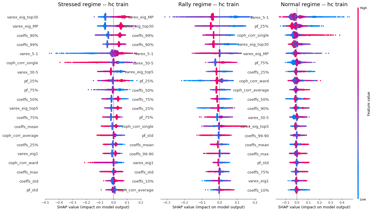
display_shap_per_class(features_train, sample_type='hc train')
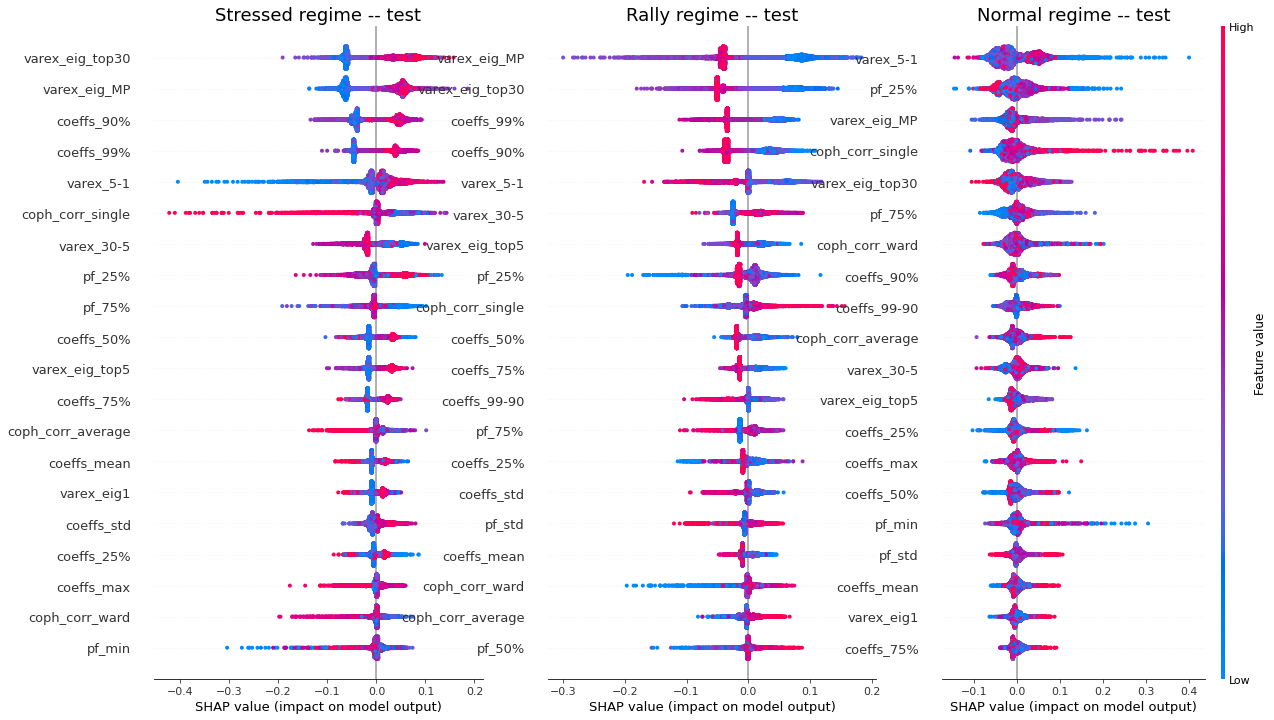
display_shap_per_class(X_test, sample_type='test')
display_shap_per_class(features_test, sample_type='hc test')
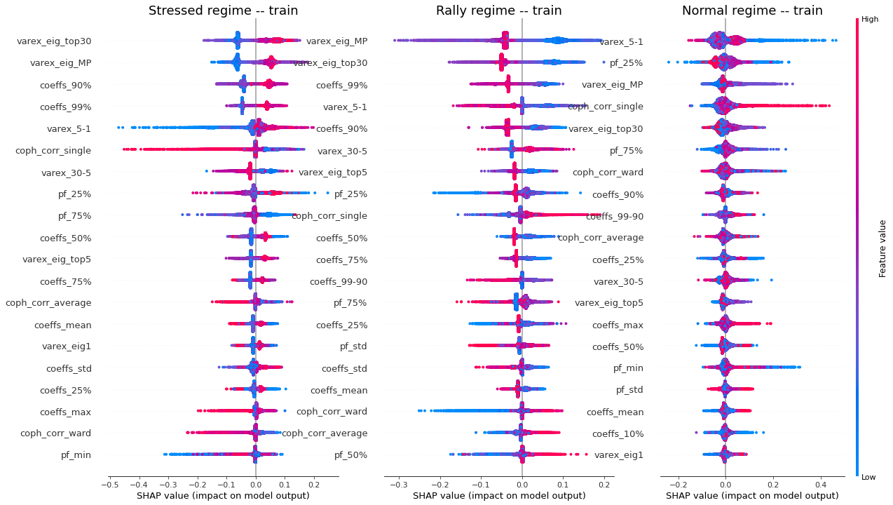
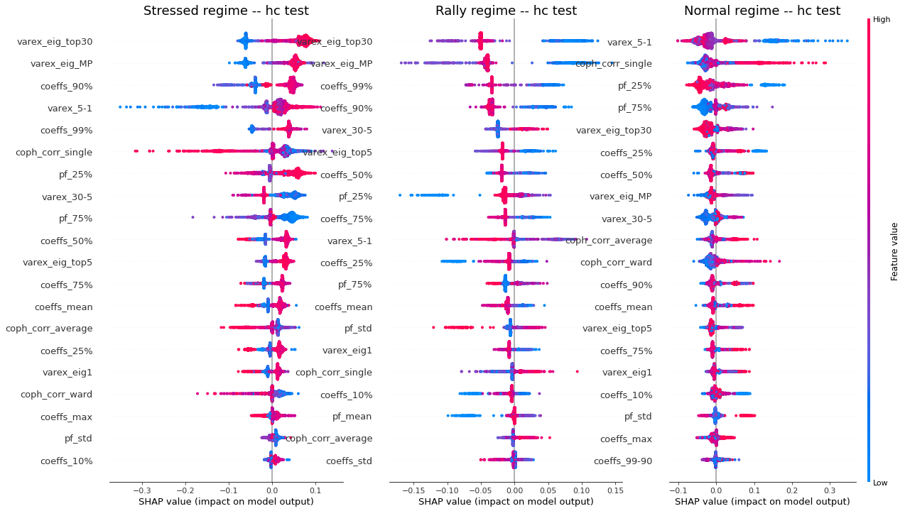
Remarks: We can notice the following:
- high values of coph_corr_single tend to inhibit the prediction of the ‘stressed’ class, i.e. when there is a strong hierarchical structure, the ‘stressed’ regime is less likely
- high values of coph_corr_single tend to push the prediction toward the ‘normal’ class, i.e. when there is a strong hierarchical structure, the ‘normal’ regime is more likely
- low values of varex_5-1 tend to push the prediction toward the ‘normal’ class; we saw that on the distribution of this feature: the ‘normal’ class has a mode localized at a low value outside the support of the two other classes
- low values of varex_5-1 tend to strongly inhibit the prediction of the ‘stressed’ class
- low values of var_eig_MP tend to push the prediction toward the ‘rally’ class, i.e. when the variance explained by the top statistically meaningful principal components is low, the ‘rally’ regime is more likely; once again, we could have guessed from the features distributions displayed in the EDA
- var_eig_top30 has a polarizing effect on both the ‘stressed’ and ‘rally’ classes, but not on the ‘normal’ one; high values of the feature tend to push the prediction toward the ‘stressed’ class, and low values tend to push it away; the converse for the ‘rally’ class
Can we build a good model with only 2 features?
Based on all the previous observations, one can wonder if we can make a decent model with 2 features only?
feat1 = 'varex_eig_MP'
feat2 = 'coph_corr_single'

clf = RandomForestClassifier(random_state=42)
clf.fit(X_train[[feat1, feat2]], y_train)

features_train, labels_train = get_high_confidence(
    X_train[[feat1, feat2]], y_train)
features_test, labels_test = get_high_confidence(
    X_test[[feat1, feat2]], y_test)

print('Accuracy on the train set: \t',
      round(clf.score(X_train[[feat1, feat2]], y_train), 2))
print('Accuracy on the train set when the model has high confidence: \t',
      round(clf.score(features_train[[feat1, feat2]], labels_train), 2))
print('Accuracy on the test set: \t',
      round(clf.score(X_test[[feat1, feat2]], y_test), 2))
print('Accuracy on the test set when the model has high confidence: \t',
      round(clf.score(features_test[[feat1, feat2]], labels_test), 2))
Accuracy on the train set: 	 1.0
Accuracy on the train set when the model has high confidence: 	 1.0
Accuracy on the test set: 	 0.66
Accuracy on the test set when the model has high confidence: 	 0.88
That is, compared to the model trained using the 45 available features, a decrease in accuracy of 66 / 80 - 1 = -17.5% on the test set.
Let’s just check visually how well the two features are separating the classes in the 2D plane:
def plot_feat2d(features, labels, feat1, feat2, fig_title='',
                nr=2, nc=2, idx=1, disp_normal=True):
    data = pd.concat([features, labels], axis=1)
    plt.subplot(nr, nc, idx)
    tg = 'stressed'
    plt.scatter(data[data['target'] == tg][feat1],
                data[data['target'] == tg][feat2],
                alpha=0.2, label=tg, color='red')
    tg = 'rally'
    plt.scatter(data[data['target'] == tg][feat1],
                data[data['target'] == tg][feat2],
                alpha=0.2, label=tg, color='green')
    if disp_normal:
        tg = 'normal'
        plt.scatter(data[data['target'] == tg][feat1],
                    data[data['target'] == tg][feat2],
                    alpha=0.2, label=tg, color='blue')
    plt.xlabel(feat1)
    plt.ylabel(feat2)
    plt.legend()
    plt.title(fig_title)
plt.figure(figsize=(18, 12))
plot_feat2d(X_train, y_train, feat1, feat2,
            fig_title='Train dataset', idx=1, disp_normal=False)
plot_feat2d(features_train, labels_train, feat1, feat2,
            fig_title='Subset of Train dataset where model has high confidence',
            idx=2, disp_normal=False)

plot_feat2d(X_test, y_test, feat1, feat2,
            fig_title='Test dataset', idx=3, disp_normal=False)
plot_feat2d(features_test, labels_test, feat1, feat2,
            fig_title='Subset of Test dataset where model has high confidence',
            idx=4, disp_normal=False)
plt.show()
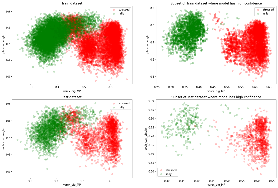
The two classes ‘stressed’ and ‘rally’ are nearly (even linearly) separable in the 2D plane (varex_eig_MP, coph_corr_single).
plt.figure(figsize=(18, 12))
plot_feat2d(X_train, y_train, feat1, feat2,
            fig_title='Train dataset', idx=1)
plot_feat2d(features_train, labels_train, feat1, feat2,
            fig_title='Subset of Train dataset where model has high confidence',
            idx=2)


plot_feat2d(X_test, y_test, feat1, feat2,
            fig_title='Test dataset', idx=3)
plot_feat2d(features_test, labels_test, feat1, feat2,
            fig_title='Subset of Test dataset where model has high confidence',
            idx=4)
plt.show()
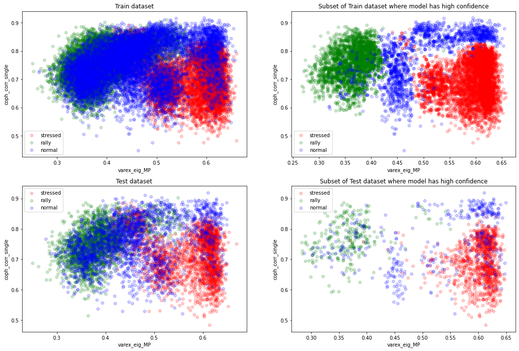
However, we can see that the ‘normal’ regime distribution support is overlapping a lot with the other two classes, and especially with the ‘rally’ one.
We can also observe that the accuracy of 1 we obtain on the training set is suspicious and suggests some overfitting since there is the fundamental Bayes error rate that should come into play.
From the above graphs, we can think that a 4-component Gaussian mixture model would do a good job (at simplifying the decision boundaries).
def plot_feat2d_proba_level(features, feat1, feat2,
                            nr=2, nc=2, idx=1,
                            fig_title=''):
    proba = clf.predict_proba(features[[feat1, feat2]])
    plt.subplot(nr, nc, idx)
    cm = plt.cm.get_cmap('RdYlBu')
    sc = plt.scatter(features[feat1],
                     features[feat2],
                     c=proba.max(axis=1),
                     vmin=0,
                     vmax=1,
                     s=50,
                     cmap=cm)
    plt.colorbar(sc)
    plt.xlabel(feat1)
    plt.ylabel(feat2)
    plt.title(fig_title)
plt.figure(figsize=(18, 12))
plot_feat2d_proba_level(X_train, feat1, feat2, idx=1,
    fig_title='Model confidence on Train dataset')
plot_feat2d_proba_level(features_train, feat1, feat2, idx=2,
    fig_title='Model confidence on High-Confidence-Train dataset')
plot_feat2d_proba_level(X_test, feat1, feat2, idx=3,
    fig_title='Model confidence on Test dataset')
plot_feat2d_proba_level(features_test, feat1, feat2, idx=4,
    fig_title='Model confidence on High-Confidence-Test dataset')
plt.show()
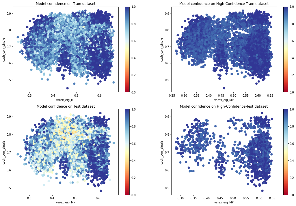
We can see that the model is less confident in the areas of overlapping distributions.
Conclusion: In this study, we show how we can use basic machine learning models such as random forests to gain more insights into a phenomenon, and maybe build a theory around it.
Concretely, we show that some features of the correlation matrix are strongly associated with the market regime (defined by the performance of a simple equi-weighted portfolio of stocks). This is an interesting result as we discard the volatility information (typically considered as the main indicator for market stress), and the returns information (used to define the ‘stressed’, ‘normal’, ‘rally’ classes).
We also show how
- looking at the conditional distribution of the features (and their correlations),
- using SHAP,
- simplifying the model to only a couple of variables (and potentially adopting a simpler model),
can help us gain confidence in either the model or the phenomenon/theory.