Some Thoughts on the Applications of Deep Generative Models in Finance

Some Thoughts on the Applications of Deep Generative Models in Finance
Thinking in progress…
Not a technical post. Just some high-level thoughts on the potential applications of deep generative models in finance.
- YouTube video: Applications of GANs in Finance

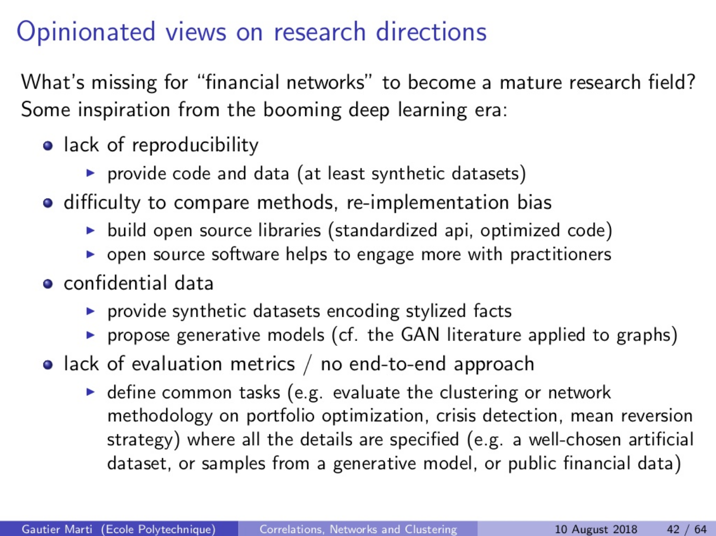
Presentations I did at various conf/webinars:
Literature review
Data Anonymisation
This paper focuses on privacy preserving generation of synthetic data (in finance): Essentially tabular data in retail banking and time series of market microstructure data. Sharing more widely banking and financial data could allow financial institutions to leverage the work of the academic community (and others), and build on their research. However, for now, restrictions are such that it is close to impossible. The paper describes three areas which need to be investigated further to meet business demand and regulatory requirements: 1) Generating realistic synthetic datasets 2) Measuring the similarities between real and generated datasets 3) Ensuring the generative process satisfies any privacy constraints. If these goals are met, financial institutions will be able to share more widely their sensitive data in guise of realistic synthetic datasets. Note that many methods based on neural networks do not guarantee privacy as these models can memorize data (some inputs can be perfectly encoded in their parameters) and restore them back in guise of the pseudo-synthetic data. $(\epsilon, \delta)$-differential privacy is the privacy framework the most widely accepted by the scientific community to study, guarantee and tune the tradeoff between noise and privacy.
Authors show that a Restricted Boltzmann Machine (RBM) is able to learn multivariate distribution of dataset features and generate new synthetic samples from the learned distribution. They claim this technique can help for data anonymisation, outlier detection and fighting overfitting. Unlike GANs (usually deep nets), RBMs (shallow nets) seem to be able to work well with small samples, and therefore might be useful for upsampling a training dataset. Larger training datasets can provide some regularization to the model one is trying to fit. Moreover, since the RBM has an autoencoder information bottleneck structure, it should generate samples without outliers helping furthermore the training of the downstream model (classification or regression). Authors try to empirically validate these intuitions using three UCI ML repository datasets (Wisconsin breast cancer, Coimbra breast cancer, Australian credit approval) and a synthetic dataset (simulated data from a known probability distribution). The UCI datasets are quite small: 569, 116, 690 samples respectively. Respective tasks are binary classification. Authors show that ML models trained on the synthetic data generated by the RBM perform on par with the ones trained on the original data. Moreover, in the case of the smallest dataset where features are also less predictive, synthetic-data trained ML models are actually outperforming the ones trained on the original data. This is meant to show that both data-regularization (5000 synthetic samples instead of the 116 original ones) and outlier-filtering (autoencoder information bottleneck regularization) obtained with the RBM can help fit better models. The toy-example, i.e. learning a complex multiviariate distribution with non-linear dependence, shows the limit of the RBM: It becomes data-hungry, and even with reasonably large sample sizes it fails to capture fully the distribution. Authors claim their approach has good data anonymisation properties, however it is not clearly stated formally or discussed in terms of the differential privacy formalism.
In this short note, authors observe that many studies and economic analyses cannot be replicated due to the sensitive or proprietary nature of the data being used. The reader is left to believe the results exposed, which is contrary to the scientific approach. (Deep) generative models for synthetic data generation can be a solution to share anonymized datasets between economists. An ideal workflow would roughly look like this: 1. Describe the true sensitive/proprietary/private data; 2. Describe the synthetic data generating model which has produced the synthetic dataset; 3. Run the same analyses on both the true and synthetic data; 4. Confirm that results on both datasets are comparable; 5. Publicly release the synthetic dataset. Authors list a couple of generative models for synthetic data: The Synthetic Data Vault (based on multivariate Gaussian copulas); Auto-encoder based techniques (some of which are differentially private, but can still be susceptible to model inversion and GAN-based attacks); Generative Adversarial Networks (GANs); Autoregressive models; Normalizing Flow models; Energy-based models. These models can be useful to redesign standard Monte Carlo studies, and robustness checks to confirm that perturbing the true data (when generating synthetic data) does not break results.
Modeling and Generating Financial Time Series
(e.g. financial assets returns)
Authors advocate for the use of Conditional Generative Adversarial Networks (cGANs) to learn and simulate time series data with financial risk applications in mind. Authors notably show that Value-at-Risk (VaR) and Expected Shortfall (ES) estimates obtained from cGAN simulations are more accurate than the ones obtained from the standard historical simulations, meaning that cGAN-based estimates are closer to the realized values (number of VaR breaches is about right for cGAN whereas VaR is underestimated for historical simulations leading to a too high number of VaR breaches; cGAN-based ES is close to the actual ES whereas historical simulations based ES is underestimated). Authors also show that a conditional GAN could be used as an economic forecasting model, a compelling alternative to large-scale econometric models like MAUS (Macro Advisers US Model) which can only produce a single forecast for a given condition whereas a cGAN model can generate a forecast distribution. Besides working with real financial data (two stocks time series for the VaR example, and unemployment rate, GDP time series for the macroeconomic use case), authors discuss at length the ability for a cGAN to recover an underlying known data generative process: 1. Gaussian Mixture Models; 2. VAR models with switching regimes (approx. macroeconomic index data); 3. GARCH models (approx. 1-day stock returns). cGANs are able to recover the underlying model well (at least matching statistics). However, it depends (quite obviously) on the sample size… Practitioners, beware!
Authors propose to use a conditional GAN (cGAN) for fine-tuning trading strategies, and ensembling models. Basically, the first step is to fit a conditional GAN to a (set of) time series of interest. This is no trivial task as GANs are notoriously known for being hard to train. Authors show a few failed attempts: With too few epochs (200), generated time series are not realistic; With too many epochs (5000), generated time series are not realistic either; With approximately 1000 epochs, authors have been able to obtain convincing results (ACF and PACF of the generated time series are very similar to the original ones). Once a decent cGAN model $G$ has been built, one can use it to sample new synthetic time series. For the fine-tuning trading strategies use case, $B$ synthetic time series are generated, and then each one is split in a training set and a validation set (contiguous blocks) on which a set of hyperparameters are evaluated. One should pick the hyperparameters which maximize the average performance on the $B$ validation time series. For ensembling models, the process is rather similar: Given a good cGAN, generate $B$ synthetic time series, then train a model $M_{\lambda}^{(b)}$ on each of the $B$ samples, and finally return $M_{\lambda}^{(1)}, \ldots, M_{\lambda}^{(B)}$. The use of a cGAN (various model size) for sampling alternative paths is empirically compared to the stationary bootstrap. Authors find that a cGAN can help enhance systematic trading strategies performance (in terms of cumulative returns, Sharpe and Calmar ratios).
Authors show that it is possible to generate realistic financial (univariate) time series using a vanilla GAN with multilayer perceptron (MLP) architecture for the generator $G$ and the discriminator $D$. In order to evaluate the results, author verify that six well-known stylized facts hold true in the generated time series. It appears that, according to their experiments, only MLP-GAN is able to recover the six stylized facts (linear unpredictability; heavy-tailed distribution; volatility clustering; leverage effect; coarse-fine volatility correlation; gain/loss asymmetry) in its generated synthetic time series. Competing approaches such as stochastic processes (GARCH, EGARCH) or agent-based models are not able to generate time series which verify all of the above stylized facts. Authors also show that using alternative architectures for the GAN such as CNN, MLP-CNN, or even MLP with batch normalization, they were not able to capture the six stylized facts.
Authors propose an alternative architecture for the two competing neural networks inside a GAN: Instead of the standard multilayer perceptrons (MLPs), they suggest to use Temporal Convolutional Networks (TCNs). Empirical studies have shown that TCNs are competitive with typical recurrent architectures, and can be even better at capturing long-range dependencies as they do not suffer from the vanishing and exploding gradients problem. Their main drawback is that their range (sequence length) is by construction bounded (unlike recurrent architectures which can in theory - but not in practice - capture all past information). It is possible to extend their range with a larger network and therefore more parameters but then it is questionable whether there is enough data available to train them meaningfully. Despite this limitation, they have been found to outperform LSTMs on supervised learning benchmarks. Interestingly, authors demonstrate that a vanilla GAN cannot generate heavy-tails by showing that all moments exist (i.e. are finite). This result also extends to their model, an undesirable property since financial time series are known for their heavy-tails. To circumvent this problem, authors suggest to learn the inverse Lambert W probability transform of the original log returns which has lighter tails. The Lambert W probability transform being bijective, light-tailed generated stock returns can be made heavier by applying the reciprocal function. Besides proposing to use a TCN-GAN, authors also introduce a stochastic volatility neural network, i.e. a TCN which models the volatility and drift $(\sigma_{t, \theta}, \mu_{t, \theta})$ processes and a mere network which models the innovations $\epsilon_t, \theta’$ which are independent. This construction allows the authors to derive the transition to the risk-neutral distribution. Finally, in guise of numerical experiments, authors aim to model the log returns of the S&P 500. They compare a pure TCN-GAN, their stochastic volatility neural network GAN and a GARCH(1, 1). To evaluate the quality of the synthetic data generated, authors use several metrics: essentially distributional metrics (e.g. Earth Mover Distance) and dependence scores (e.g. ACF). They find that the pure TCN-GAN performs the best, closely followed by their stochastic volatility neural network GAN. The GARCH model performs poorly in comparison. Interestingly, authors conclude that “a single metric needs to be developed which unifies distributional metrics with dependence scores we used in this paper and allows to benchmark different generator architectures”. I struggled myself quite a bit on this question of combining these two pieces of information (dependence and distribution) during my PhD on clustering with copula-based distances. Note that the ‘dependence’ authors have in mind here is the temporal (or serial) dependence, but in the multivariate setting (the 500 constituents of the S&P 500, for example) one has also to deal with the much more complex cross-sectional dependence (cf. CorrGAN)…
Authors propose to use a shallow generative neural network – a Restricted Boltzmann Machine (RBM) – to generate realistic synthetic market data. They first show that a RBM is able to recover well toy-example (a mixture of two Normal distributions): The synthetic data generated by the RBM and the original data have a very similar histogram, their QQ-plot is a straight line; Matching the first two moments and sampling from a fitted Normal distribution yields much worse results. Then, authors show through various statistics (linear and non-linear correlations, volatilities, tails of the univariate margins) that a RBM is able to learn the multivariate joint distribution of spot FX rates (5070 daily log-returns of EURUSD, GBPUSD, USDJPY and USDCAD between 1999 and 2019). Using properties from the RBM, they also show how to control autocorrelation as a function of the thermalisation parameter K (K is the number of iterations between the visible and hidden units of the RBM): Lower K correponds to high autocorrelation, higher K corresponds to low or even 0 autocorrelation. They also show how it is possible to do conditional sampling and thus obtain non-stationary time series: They add a binary variable which encodes, for example, low or high volatility regime. During the training, the RBM learns the joint distribution (log-returns, volatility regime). Then, the following approach is applied for the conditional sampling: During the thermalisation phase (back and forth iterations) they constantly reset the binary variable to the chosen volatility regime, and thus obtaining samples which are likely from the targeted volatility regime.
Modeling and Generating Correlations of Financial Time Series
(e.g. correlations between stocks returns, risk premia, strategies, spreads of pairs/baskets trades)
Author (actually, me) shows that it is possible to generate realistic synthetic financial correlation matrices using a GAN. The GAN, a Deep Convolutional Generative Adversarial Network (DCGAN) architecture, is trained on a few thousands of empirical correlation matrices estimated from the S&P 500 constituents returns. Inputs (correlation matrices) are re-ordered using a hierarchical clustering algorithm to obtain a ‘canonical’ representation and help the learning process to be more data efficient (there are n! permutations of the rows/columns). Outputs, which may not be exactly PSD, are projected on the elliptope (the space of correlation matrices). The author shows that correlation matrices obtained verify six well-known stylized facts of financial correlation matrices. It still remains to be shown whether the GAN is able to sample from the full empirical subspace of the elliptope or is suffering from a mode collapse, and therefore only able to sample from a small part of the empirical subspace. Potential applications: Simulations for comparing portfolio allocation methods (assets or alphas/strategies); Simulations for testing concentration risk of a portfolio of pair trades (mean-reverting baskets), etc.
Modeling and Generating Tabular Datasets
(e.g. alternative data)
In this paper, researchers from the ‘Credit and Fraud Risk’ department at American Express show how to use GANs to generate realistic synthetic (anonymized) versions of highly sensitive and confidential American Express datasets. Authors acknowledge the fact that modern machine learning progress was driven by the shared corpus of publicly available datasets which are used as benchmarks to validate novel ML algorithms. However, publicly available finance-related datasets do not exist to help researchers in financial machine learning since they are most often than not very confidential. This lack of common benchmarks slows down research progress, and possibly American Express would like to piggyback on academic research to improve its models for i) assessing creditworthiness of customers, ii) offering customers optimal financial products, and iii) identifying fraud. A potential solution could be to publicly share anonymized synthetic versions of the real data provided they are realistic enough. Authors find that a well-trained GAN is able to replicate the distribution of the original data (three American Express tabular datasets containing numerical and categorical features, and a target variable which can be continuous or binary). Authors find that pre-processing the features helps for training the GAN. They evaluate their results by checking three criteria: i) the distribution of individual features (which can be skewed, binary, discrete or contains peaks) in generated data should match those in real data; ii) the overall distributions of generated and real data should match; iii) the relationship between features and the target variable in real data is replicated in generated data. They find that their GAN generates data which satisfy the three criteria, but notice that out-of-sample performance on downstream ML tasks is slightly worse for models trained on synthetic data rather than the original one.
Modeling and Generating Transactions
(e.g. sequence of trades on various instruments)
This paper proposes to use a GAN based model to estimate the probability that a large transfer is fraudulent. It outperforms well-known classification methods according to its authors, and its application has reduced losses in two Chinese commercial banks where it is deployed. The GAN is actually encompassing a denoising autoencoder where the encoder is part of the discriminator and the decoder is part of the generator. The latent representation $z$ of the features is used both as an input to the generator, and as an input to a Gaussian Mixture Model (GMM) which outputs a score quantifying how likely the input transfer $x$ is a normal transfer rather than a fraudulent one. This hybrid model (GAN/autoencoder) seems to give the best performance on this classification task (in terms of precision, recall, fall-out).
Not directly a finance-focused paper, but it is not hard to see that the business problem exposed (generating synthetic realistic orders that could have been made in a e-commerce website) is quite similar to product placements in retail/commercial banking, and insurance industries. Otherwise, the paper is a collection of good practical ideas and insights on the implementation of such a GAN-based system. Many techniques are employed for doing 1) product embeddings (an inverse-document-frequency-weighted-average of word2vec representations for the words in the product descriptions); 2) customer embeddings (obtained using a neural network trained on multi-task predictions: a) predicting the next product group purchased by a customer; b) predicting how much price a customer will pay on the next purchase; c) predicting after how many days the customer will purchase an item again); price (log-transformed and normalized), and date of purchase (unit circle (cos, sin) representation), are more straightforward to encode as features. An order (product, customer, price, date of purchase) is represented by a vector $x \in [-1, 1]^{264}$. The Wasserstein GAN and conditional Wasserstein GAN used are standard (discriminator and generator are MLPs), but there is an interesting discussion about the hyperparameters and their impact on the training stability and quality of the results obtained. Quality of the results is assessed in several different ways (some quite innovative and rather astute): t-SNE; feature correlation; data distribution in Random Forest leaves. Applications: Given a new product, the synthetic orders can be used to characterize the customers who will buy this product, what should be the price of this product, and any seasonality in the demand. This information can be used to manage inventories and proactively optimize the supply chain.
Following the seminal work exposed in eCommerceGAN: A Generative Adversarial Network for E-commerce, authors propose a GAN-based method to generate customer-level transactions. Unlike the previous work which generates realistic orders for a given product, this novel method aims at directly modelling customer behaviour over time. Similarly to the previous work, authors use a multi-task LSTM to obtain customer embeddings. The LSTM is trained to predict a) whether or not a product is the last product in the basket; b) the category of the next product; c) the price of the next product. Product embeddings are obtained from their textual descriptions using a Word2Vec model. Then, a conditional Wasserstein GAN with gradient penalty (cWGAN-GP) is trained to learn the distribution of products given a customer (embedding) and a week. The cWGAN-GP, if trained correctly, should be able to generate realistic product embeddings. If one wants to obtain real-world products rather than embeddings (for example, in the case of product recommendations to a customer $h$ for week $w$), one can look for the product $p$ in the database of real-world products whose embedding minimizes the distance to the generated embedding, i.e. . To generate a sequence of baskets of products that a customer will likely purchase over several consecutive weeks, the process works as follow: Given a customer and his transaction history $B_1, B_2, \ldots, B_i$, where each $B_i$ denotes a basket for week $w_i$, the method generates a basket $B_{i+1}$ for the following week by sampling from $G(z | (h_i, w_i))$. The embedding $h_i$ of the customer at week $w_i$ is obtained by passing the sequence $B_1, B_2, \ldots, B_i$ through an LSTM and extracting the hidden state. Thus, generating longer purchase sequences is straightforward: Feed $B_{i+1}$ through the LSTM, extract the updated customer embedding $h_{i+1}$ as if the customer had purchased $B_{i+1}$, sample $B_{i+2}$ from $G(z | (h_{i+1}, w_{i+1}))$, etc. Concerning validation of their results, authors i) check feature distributions; ii) show that the top most common real sequential patterns (subsequences of items across baskets customers have bought over time) are also found in the generated data; iii) project real and generated baskets (as bag-of-products vectors) onto the plane using t-SNE and a PCA qualitatively indicating that the distributions match closely; iv) train a logistic regression to distinguish between real and generated baskets. A perfectly indistinguishable generated dataset should yield a classification accuracy of 50%. Authors obtain a classification accuracy of 63%.
Modeling and Generating Accounting & Financial Statements
(e.g. journal entries in Enterprise Resource Planning (ERP) systems)
Authors investigate the use of Adversarial Autoencoders (AAEs), a hybrid architecture built from an autoencoder and a generative adversarial network, for detecting and understanding accounting anomalies. Standard techniques applied by forensic accountants consist in using handcrafted rules derived from known fraud scenarios, which fraudsters may gradually find ways to circumvent. Authors use the properties of AAEs to i) learn representations of journal entries which are clustered into semantic meaningful groups; ii) sample journal entries for an audit in an interpretable manner; iii) a novel anomaly score. Authors tell us that there are two classes of anomalous journal entries: Global accounting anomalies, which are unusual or rare individual attribute values (they are usually errors rather than frauds); Local accounting anomalies, which are an unusual or rare combination of attribute values while their individual attribute values occur quite frequently (such anomalies have a high chance to be associated to fraud). From a proba/stat point of view, the global anomalies correspond to outliers in the marginals (the univariate distribution of the variables/features) which are rather obvious to detect and therefore not likely to be introduced by fraudsters. The local anomalies, on the other hand, are outliers with respect to the joint distribution of variables/features, and therefore harder to find for an auditor. AAEs allow to detect both classes of anomalies in an unsupervised manner. Adversarial Autoencoders (AAEs) are autoencoders whose latent space (the encoded variable) is constrained to follow a given distribution. This constraint is enforced by a GAN whose discriminator is tasked to distinguish between samples of the autoencoder latent space (considered as output from a generator) and samples from the prescribed distribution. The autoencoder, trained to reconstruct its input, is thus forced to encode the dataset into vectors following the prescribed distribution (rather than being placed arbitrarily in the latent space or centered around a single mode as in the case of a standard variational autoencoder (VAE)). Authors choose a simple mixture of isotropic Gaussians $\mathcal{N}(\mu_k, I)$, with $k=1, \ldots, 10$, as the prescribed distribution. If the training of the AAE is successful, similar journal entries should be encoded close to the same mode in the latent space. Thus, each mode should capture journal entries with similar characteristics. Outliers, or accounting anomalies, are either samples far from any mode or samples whose reconstruction error is high. The former case tends to be associated with global accounting anomalies (usually errors) while the latter case tends to be associated with local accounting anomalies (usually frauds). Authors define an anomaly score which is a convex combination of the normalized mode divergence and the normalized reconstruction error. For experiments, authors use two datasets of journal entries and inject synthetic local and global anomalies (less than 0.03% of total entries). Like many other researchers, authors notice that the training of such an architecture is hard and unstable: “we face a variety of collapsing and non-convergence scenarios.” Provided a good set of hyper-parameters is found, authors show that their method is able to find accounting anomalies in an unsupervised way, and partition the journal entries into semantic clusters which allow auditors to sample and analyze journal entries in an interpretable manner. GitHub code is available: https://github.com/GitiHubi/deepAD
In this paper, the authors explore the application of Deepfakes (typically fake videos of people) to Accounting. This set of techniques could be applied by fraudsters to fool both the usual rule-based Computer Assisted Audit Techniques (CAATs) and statistical CAATs. The main idea is to use an Adversarial Autoencoder to learn a disentangled and simple latent representation of the space of journal entries. The GAN part is used to regularize the latent space of the autoencoder, and to impose some structure on it. The prior is chosen to be regularly spaced isotropic 2d Gaussians. Why such a choice? Authors claim that the journal entries have a natural hierarchical structure, so why not organizing the isotropic Gaussians hierarchically? Authors find the latent space is well disentangled: Each isotropic Gaussian captures a high-order latent factor of variation, e.g. business process or organizational function; Inside each Gaussian, a low-order latent factor of variation is expressed, e.g. posting amounts. Authors use the latent space regularity to sample fake journal entries along well-chosen paths to generate expected and realistic values which are coherent altogether. The two main strategies are: i) replace a big fraudulent transaction with lots of smaller ones to fool rule-based CAATs which may red-flag a big amount; ii) add fake journal entries to hide the fraudulent one so that it does not stand out as a statistical anomaly for the statistical CAATs.
No GANs in this paper, but a Vector Quantised-Variational Autoencoder (VQ-VAE), that is a VAE whose latent space is discrete and supported by a given number of vectors (a codebook of embedding vectors). There are a couple of technical tricks to train these models, e.g. the stop-gradient operator. The “business” problem is the following: Auditors have to assess and certify that the financial statements are a ‘true and fair presentation’ of the companies. The trustworthiness of these financial statements is paramount for investors and creditors, and the economy. The assessment has to be based on the journal entries, that is the list of debit and credit between the various accounting ledgers of a financial statement. Nowadays, the number of these journal entries is huge, and it can be close to impossible to assess fully. Audit sampling has thus become a common practice, ie the ‘selection and evaluation of less than 100% of the entire population of journal entries’. Audit sampling increases the efficiency of a financial audit, but it also increases its sampling risk, ie the risk that the auditor’s conclusion based on auditing a subset of entries may differ from the conclusion of auditing the entire population. Auditors are required to select a representative sample from the population of journal entries to mitigate sampling risks. But, what does it mean concretely??? It does not seem easy to do! In fact, solutions applied in the industry are naive, at best. Authors of the paper propose to use a VQ-VAE to learn representative samples from vast quantities of journal entries, which are also interpretable by human auditors. Each embedding vector of the codebook can capture an underlying business process or workflow. Authors apply their approach on two publicly available datasets: i) payments data of the City of Philadelphia’s fiscal year 2017; ii) vendor payments of the City of Chicago from 1996 to today. They empirically find that the VQ-VAE is able to uncover the latent generative factors (represented by the learned embeddings) which are, for example, fleet management (auto parts), legal services (appointed attorneys), office materials and supplies, professional services (consultancy), fuel and gasoline payments, public transport maintenance, family assistance services (homeless financial support), aviation maintenance, IT services, water management, library services payments, etc. These “clusters” of journal entries are representative and human interpretable samples which match closely business processes and workflows; They should reduce sampling risks of audits. Authors also mention that disentanglement (of the latent space) has no unique and widely accepted definition yet. Thus, they evaluate their results using four different metrics: $\beta$-VAE metric, Factor-VAE metric, Mutual Information Gap (MIG), Disentanglement Metric (DCI). They find that the disentanglement increases with the codebook size (the number of embedding vectors used to quantize the posterior). Question: How does this quantization compare with a K-means on the latent space?