Back to basics: PCA on stocks returns
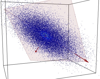
Principal component analysis Image from Gael Varoquaux blog
Back to basics: PCA on stocks returns
A short code snippet to apply PCA on stocks returns. No secret sauce is used here to clean the empirical covariance matrix. This blog post will mostly serve as a basis for comparing several flavours of PCA and their impact on ex-ante volatility estimation. We may look in future blog posts into Sparse PCA, Nonlinear PCA, Kernel PCA, Robust PCA, revisit our previous implementation of Hierarchical PCA (HPCA), and other techniques such as Independent Component Analysis (ICA).
from pathlib import Path
from datetime import datetime
import numpy as np
import pandas as pd
from tqdm import tqdm
from pandas.tseries.offsets import BDay
from sklearn.linear_model import LinearRegression
import matplotlib.pyplot as plt
sp500 = pd.read_csv('SP500_HistoTimeSeries.csv',
                    index_col='Date',
                    date_parser=lambda x: datetime.strptime(x, '%d/%m/%Y'))
sp500.index = pd.to_datetime(sp500.index)
sp500 = sp500.sort_index()
returns = sp500.pct_change()
returns = returns.clip(lower=-0.25, upper=0.25)
del returns['SPX Index']
NB_EIGEN = 5
LOOKBACK_WINDOW = 2 * 252
dates = returns.index[LOOKBACK_WINDOW:]
factor_covariances = []
factor_exposures = []
residual_vols = []

for date in tqdm(dates):
    # compute the PCA on rolling past returns
    past_returns = returns.loc[date - BDay(LOOKBACK_WINDOW):date]
    past_returns = past_returns[(past_returns.count() > 100)
                                .replace(False, np.nan)
                                .dropna()
                                .index]
    cov = past_returns.cov()
    eig_vals, eig_vecs = np.linalg.eig(cov)
    permutation = np.argsort(-eig_vals)
    eig_vals = eig_vals[permutation]
    eig_vecs = eig_vecs[:, permutation]
    zeroed_returns = past_returns.replace(np.nan, 0)
    factors = zeroed_returns @ eig_vecs.real
    factors_5 = factors.iloc[:, :NB_EIGEN]
    reg = (LinearRegression(fit_intercept=True)
           .fit(X=factors_5, y=past_returns.fillna(0)))
    B = reg.coef_
    pca_returns = reg.predict(factors_5)
    resid = past_returns - pca_returns
    resid_vol = resid.std()
    D = np.diag(resid_vol)**2

    # factor covariance
    fCov = (factors_5
            .cov()
            .rename(columns={i: 'E' + str(i) for i in range(NB_EIGEN)},
                    index={i: 'E' + str(i) for i in range(NB_EIGEN)})
            .stack()
            .reset_index()
            .rename(columns={'level_0': 'factor_1',
                             'level_1': 'factor_2',
                             0: 'covar'}))
    fCov['date'] = date
    fCov = fCov.set_index(['date', 'factor_1', 'factor_2'])

    # factor exposures
    fExp = pd.DataFrame(B,
                        index=past_returns.columns,
                        columns=['E' + str(i) for i in range(NB_EIGEN)])
    fExp['date'] = date
    fExp = fExp.reset_index().rename(columns={'index': 'ticker'})
    fExp = fExp.set_index(['date', 'ticker'])

    # specific risk
    spec_risk = (resid_vol
                 .reset_index()
                 .rename(columns={'index': 'ticker',
                                  0: 'resid_vol'}))
    spec_risk['date'] = date
    spec_risk = spec_risk.set_index(['date', 'ticker'])

    # save the factor covariance, exposures, and stocks specific risk
    factor_covariances.append(fCov)
    factor_exposures.append(fExp)
    residual_vols.append(spec_risk)

factor_covariances = pd.concat(factor_covariances)
factor_exposures = pd.concat(factor_exposures)
residual_vols = pd.concat(residual_vols)
100%|██████████| 3470/3470 [24:27<00:00, 2.37it/s]
We save the factors covariance, exposures, and residual volatilities for future reuse:
Path("risk_model").mkdir(parents=True, exist_ok=True)
factor_covariances.to_parquet('risk_model/factor_covariances.parquet')
factor_exposures.to_parquet('risk_model/factor_exposures.parquet')
residual_vols.to_parquet('risk_model/residual_vols.parquet')
Loading the saved risk model components:
factor_covariances = pd.read_parquet('risk_model/factor_covariances.parquet')
factor_exposures = pd.read_parquet('risk_model/factor_exposures.parquet')
residual_vols = pd.read_parquet('risk_model/residual_vols.parquet')
factor_covariances.tail()
| covar | |||
|---|---|---|---|
| date | factor_1 | factor_2 | |
| 2016-07-29 | E4 | E0 | -0.000842 |
| E1 | 0.000078 | ||
| E2 | 0.000133 | ||
| E3 | -0.000007 | ||
| E4 | 0.002611 |
factor_exposures.tail()
| E0 | E1 | E2 | E3 | E4 | ||
|---|---|---|---|---|---|---|
| date | ticker | |||||
| 2016-07-29 | XEC UN Equity | 0.068088 | -0.108401 | 0.040181 | 0.003394 | -0.173384 |
| ZTS UN Equity | 0.037352 | 0.036895 | -0.015819 | -0.090589 | -0.037028 | |
| DLR UN Equity | 0.019566 | 0.026160 | 0.081157 | 0.001729 | 0.017967 | |
| EQIX UW Equity | 0.034544 | 0.045924 | 0.033238 | -0.006657 | -0.018939 | |
| DISCK UW Equity | 0.052699 | -0.012641 | 0.002077 | 0.010083 | 0.039095 |
residual_vols.tail()
| resid_vol | ||
|---|---|---|
| date | ticker | |
| 2016-07-29 | XEC UN Equity | 0.012693 |
| ZTS UN Equity | 0.013028 | |
| DLR UN Equity | 0.009801 | |
| EQIX UW Equity | 0.011945 | |
| DISCK UW Equity | 0.014904 |
We now apply the risk model through history on a long-only equally weighted portfolio:
backtest_dates = sorted(residual_vols.index.get_level_values(0).unique())
# long-only equally weighted portfolio
weights = pd.DataFrame(False, index=returns.index, columns=returns.columns)

for date in tqdm(backtest_dates):
    weights.loc[date, residual_vols.loc[date, :].index] = True

weights = weights.astype(int)
weights = (weights
           .div(weights.sum(axis=1), axis=0)
           .replace(0, np.nan))
100%|██████████| 3470/3470 [02:30<00:00, 23.05it/s]
rets = (weights * returns.shift(-1)).sum(axis=1).loc[backtest_dates]
realized_vol = rets.rolling(63).std()
rets.cumsum().plot(
    title=f"Sharpe: {round(rets.mean() * np.sqrt(252) / rets.std(), 2)}")
plt.show()
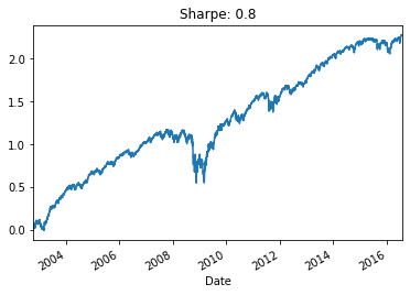
Performance and Sharpe ratio of the equally weighted long-only portfolio
pca_risk = []
for date in tqdm(backtest_dates):
    w = weights.loc[date].dropna()
    r = residual_vols.loc[date, :]
    e = factor_exposures.loc[date, :]
    c = (factor_covariances
         .loc[date, :, :]
         .reset_index()
         .pivot(index='factor_1',
                columns='factor_2',
                values='covar'))
    cov = e @ c @ e.T + np.diag(r.resid_vol**2)
    risk =  np.sqrt(w.T @ cov @ w)
    pca_risk.append(risk)

pca_risk = pd.Series(pca_risk, index=backtest_dates)
100%|██████████| 3470/3470 [01:03<00:00, 54.44it/s]
(pca_risk * np.sqrt(252)).plot( label='2y-PCA model risk')
(realized_vol * np.sqrt(252)).plot(label='3m realized risk')
plt.legend()
plt.show()
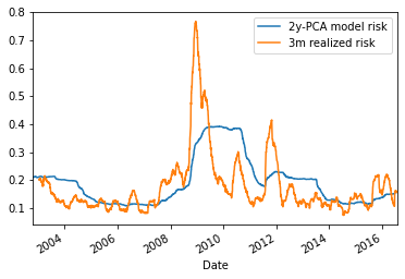
time series of the 3-month realized volatility (orange), and the *ex-ante* volatility (blue) given by the 2-year 5-factor PCA risk model
On average the 5-factor PCA risk model overestimates the risk by 5%:
(realized_vol / pca_risk).plot()
round((realized_vol / pca_risk).mean(), 2)
0.95
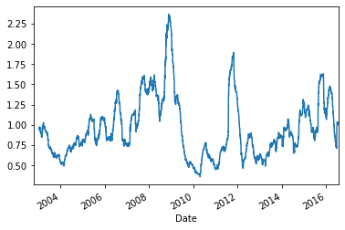
time series of the ratio between 3-month realized volatility over *ex-ante* volatility given by the 2-year 5-factor PCA risk model
We can see on the graph above that the 5-factor PCA risk model applied to such a simple long-only portfolio can be off by a factor 2 in case of extreme vol in the markets. Following a crisis, the risk model will be too conservative for a while… The duration of that period matches roughly the window length used for the PCA calibration (i.e. the rolling window size used to estimate the covariance between the stocks returns).