Naive modelling of Matalan defaulting on its MTNLN 9.5 01/31/24 Notes
Naive modelling of Matalan defaulting on its MTNLN 9.5 01/31/24 Notes
When reading Denev’s book Probabilistic Graphical Models – A New Way of Thinking in Financial Modelling, commented on my blog back in Summer 2020, I put a note in my todo list to model Matalan probability of default using a Bayesian network (for fun, not work).
I was rather familiar with this single name, former member of the iTraxx Crossover index, which had been a target for orphaning (cf. this FT article for more details).
Since then, the CDS triggered: The EMEA DC has determined that a Bankruptcy Credit Event has occurred with respect to Matalan Finance plc. due to a Chapter 15 filing (cf. this article for technical legal details).
At auction, recovery was determined at 36.5 (source creditfixings), relatively high given recent recoveries (e.g. Pizza Express at 0.125, Noble Corp at 1, Wirecard AG at 11, Diamond Offshore Drilling at 7.375, Neiman Marcus at 3, J C Penney at 0.125, …)
All that being said, the ‘23 and ‘24 notes are still performing, so far…
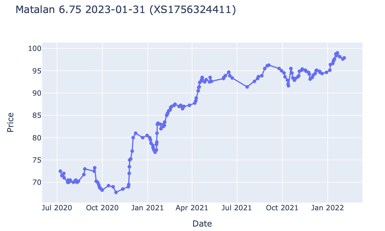
- Matalan 6.75% 2023/01/31 (senior secured, trading at 97 and yielding approximately 10% to maturity, in 1 year)
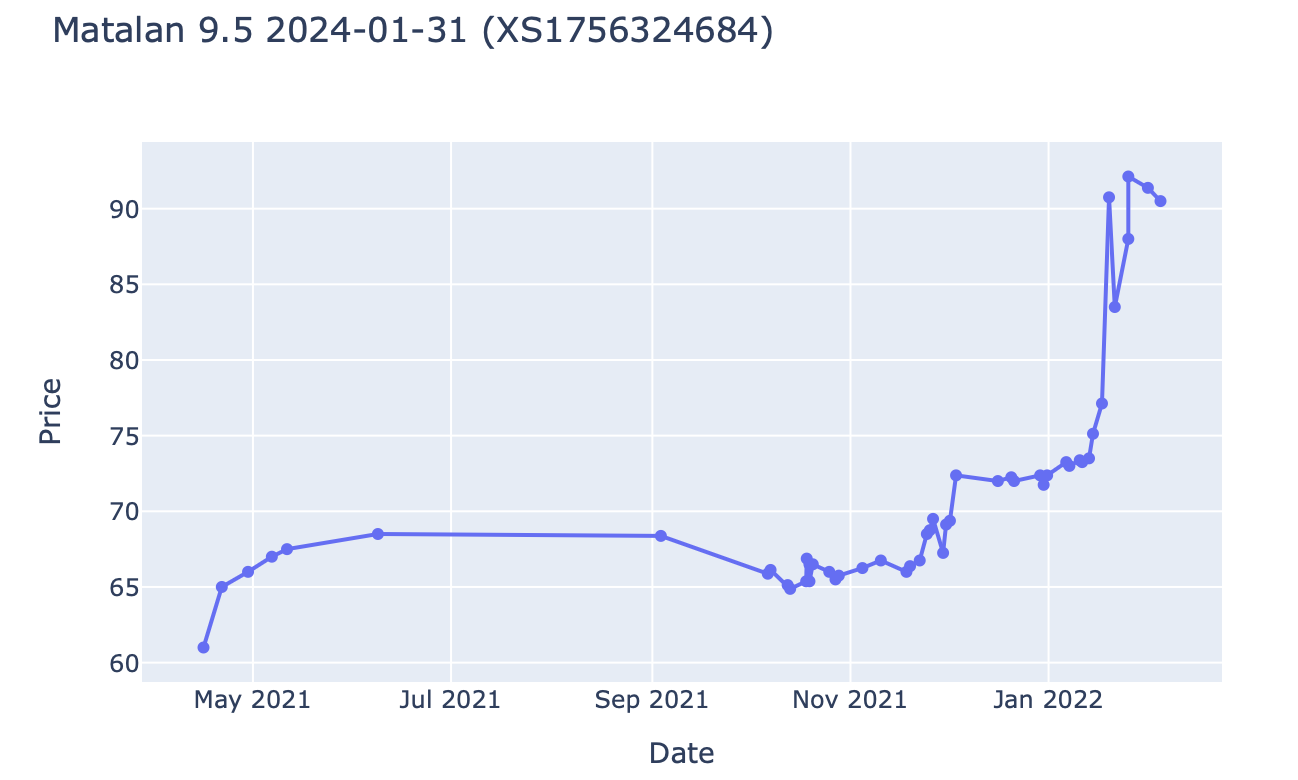
- Matalan 9.5% 2024/01/31 (second lien secured, trading at 90 and yielding approximately 15% to maturity, in 2 years)
Looking at a recent press release, and the original offering circular (from January 2018) available on WiseAlpha, we can quickly learn more about the company, its current balance sheet and income statement, and the various business risks it is exposed to.
It is not hard to see that the company is exposed to:
- disruption in its supply,
- increasing cost of goods and sales,
- increasing labour cost,
- change in customer behaviour,
- unseasonal weather (e.g. cannot sell winter clothes if warm outside; slowdown in sales at full margin followed by markdowns at the end of the season),
- data privacy laws (customer database for effective marketing),
- data leaks and reputational damage,
- depreciation of the British pound vs. USD as revenues are in GBP but costs are in USD (not fully hedged),
- organized strikes by unionized employees,
- closed shops due to COVID-19 lockdowns
- …
Based on this information, we can design a Bayesian network to estimate the probability of Matalan defaulting on its 2023 and 2024 Notes.
tl;dr This blog post is just a simple exploration of another PGM / BN library (this time pyAgrum, following the adaption of my previous blog by its authors) using a toy model inspired by credit markets.
Based on this very limited exercise, I prefer pyAgrum to pypgm in terms of user experience.
Disclaimer: Nothing in this blog should be construed as investment advice. Numbers are not based on any serious studies, and are most likely not predictive of future outcomes.
import pyAgrum as gum
import pyAgrum.lib.notebook as gnb
import pyAgrum.lib.mn2graph as m2g


bn = gum.BayesNet('Matalan default probability')
Bayesian network definition
In the cell below, we declare the random variables, and we build the graph (DAG) structure:
variables = [
    'DFLT MTLN 24',
    'DFLT MTLN 23',
    'AUDITOR',
    'KEY MGMT',
    'LITIG',
    'FRAUD',
    'DATA LEAKS',
    'SPLY BRKN',
    'GBP CRASH',
    'STRIKES',
    'STORES LCKD',
    'WRNG WTHR',
    'INFLATION',
    'LABOUR CST',
    'BRAND DMG',
    'CST SL > 900',
    'REV > 1000',
    'EBITDA > 100',]


(default_matalan_24, default_matalan_23, auditor, key_mgmt,
 litigious, fraud, data_leaks, supply_broken, gbp_crash,
 strikes, stored_locked_down, wrong_weather, inflation,
 labour_cost, brand_damage, cost_sales, revenue, ebitda) = [
    bn.add(gum.LabelizedVariable(name, '', ['False', 'True']))
    for name in variables]

edges = [('FRAUD', 'KEY MGMT'),
         ('FRAUD', 'AUDITOR'),
         ('FRAUD', 'DFLT MTLN 23'),
         ('LITIG', 'DFLT MTLN 23'),
         ('DFLT MTLN 23', 'DFLT MTLN 24'),
         ('EBITDA > 100', 'DFLT MTLN 24'),
         ('LABOUR CST', 'EBITDA > 100'),
         ('CST SL > 900', 'EBITDA > 100'),
         ('REV > 1000', 'EBITDA > 100'),
         ('INFLATION', 'LABOUR CST'),
         ('STRIKES', 'REV > 1000'),
         ('STORES LCKD', 'REV > 1000'),
         ('WRNG WTHR', 'REV > 1000'),
         ('SPLY BRKN', 'CST SL > 900'),
         ('GBP CRASH', 'CST SL > 900'),
         ('SPLY BRKN', 'BRAND DMG'),
         ('DATA LEAKS', 'BRAND DMG')]

for edge in edges:
    bn.addArc(*edge)
print(bn)
BN{nodes: 18, arcs: 17, domainSize: 262144, dim: 94}
The model has $2^{18} = 262144$ possible states.
In the cell below, we attribute marginal and conditional probabilities to define the joint distribution. Note that, here, the probabilities are assigned following my limited intuition and understanding, but in a more serious study they should be informed by historical data whenever possible and relevant.
bn.cpt('DFLT MTLN 24')[{'DFLT MTLN 23': 0,
                        'EBITDA > 100': 0}] = [0.7, 0.3]
bn.cpt('DFLT MTLN 24')[{'DFLT MTLN 23': 0,
                        'EBITDA > 100': 1}] = [0.9, 0.1]
bn.cpt('DFLT MTLN 24')[{'DFLT MTLN 23': 1,
                        'EBITDA > 100': 0}] = [0, 1]
bn.cpt('DFLT MTLN 24')[{'DFLT MTLN 23': 1,
                        'EBITDA > 100': 1}] = [0.02, 0.98]

bn.cpt('DFLT MTLN 23')[{'FRAUD': 0,
                        'LITIG': 0}] = [0.9, 0.1]
bn.cpt('DFLT MTLN 23')[{'FRAUD': 0,
                        'LITIG': 1}] = [0.8, 0.2]
bn.cpt('DFLT MTLN 23')[{'FRAUD': 1,
                        'LITIG': 0}] = [0.05, 0.95]
bn.cpt('DFLT MTLN 23')[{'FRAUD': 1,
                        'LITIG': 1}] = [0.01, 0.99]

bn.cpt('AUDITOR')[{'FRAUD': 0}] = [0.99, 0.01]
bn.cpt('AUDITOR')[{'FRAUD': 1}] = [0.5, 0.5]

bn.cpt('KEY MGMT')[{'FRAUD': 0}] = [0.95, 0.05]
bn.cpt('KEY MGMT')[{'FRAUD': 1}] = [0.75, 0.25]

bn.cpt('LITIG')[{}] = [0.98, 0.02]

bn.cpt('FRAUD')[{}] = [0.99, 0.01]

bn.cpt('DATA LEAKS')[{}] = [0.99, 0.01]

bn.cpt('SPLY BRKN')[{}] = [0.3, 0.7]

bn.cpt('GBP CRASH')[{}] = [0.9, 0.1]

bn.cpt('STRIKES')[{}] = [0.96, 0.04]

bn.cpt('STORES LCKD')[{}] = [0.9, 0.1]

bn.cpt('WRNG WTHR')[{}] = [0.95, 0.05]

bn.cpt('INFLATION')[{}] = [0.1, 0.9]

bn.cpt('LABOUR CST')[{'INFLATION': 0}] = [0.95, 0.05]
bn.cpt('LABOUR CST')[{'INFLATION': 1}] = [0.4, 0.6]

bn.cpt('BRAND DMG')[{'DATA LEAKS': 0,
                     'SPLY BRKN': 0}] = [0.8, 0.2]
bn.cpt('BRAND DMG')[{'DATA LEAKS': 0,
                     'SPLY BRKN': 1}] = [0.6, 0.4]
bn.cpt('BRAND DMG')[{'DATA LEAKS': 1,
                     'SPLY BRKN': 0}] = [0.1, 0.9]
bn.cpt('BRAND DMG')[{'DATA LEAKS': 1,
                     'SPLY BRKN': 1}] = [0.01, 0.99]

bn.cpt('CST SL > 900')[{'SPLY BRKN': 0,
                        'GBP CRASH': 0}] = [0.5, 0.5]
bn.cpt('CST SL > 900')[{'SPLY BRKN': 0,
                        'GBP CRASH': 1}] = [0.1, 0.9]
bn.cpt('CST SL > 900')[{'SPLY BRKN': 1,
                        'GBP CRASH': 0}] = [0.15, 0.85]
bn.cpt('CST SL > 900')[{'SPLY BRKN': 1,
                        'GBP CRASH': 1}] = [0.01, 0.99]

bn.cpt('REV > 1000')[{'STRIKES': 0,
                      'STORES LCKD': 0,
                      'WRNG WTHR': 0}] = [0.2, 0.8]
bn.cpt('REV > 1000')[{'STRIKES': 0,
                      'STORES LCKD': 0,
                      'WRNG WTHR': 1}] = [0.6, 0.4]
bn.cpt('REV > 1000')[{'STRIKES': 0,
                      'STORES LCKD': 1,
                      'WRNG WTHR': 0}] = [0.65, 0.35]
bn.cpt('REV > 1000')[{'STRIKES': 0,
                      'STORES LCKD': 1,
                      'WRNG WTHR': 1}] = [0.8, 0.2]
bn.cpt('REV > 1000')[{'STRIKES': 1,
                      'STORES LCKD': 0,
                      'WRNG WTHR': 0}] = [0.5, 0.5]
bn.cpt('REV > 1000')[{'STRIKES': 1,
                      'STORES LCKD': 0,
                      'WRNG WTHR': 1}] = [0.7, 0.3]
bn.cpt('REV > 1000')[{'STRIKES': 1,
                      'STORES LCKD': 1,
                      'WRNG WTHR': 0}] = [0.95, 0.05]
bn.cpt('REV > 1000')[{'STRIKES': 1,
                      'STORES LCKD': 1,
                      'WRNG WTHR': 1}] = [1, 0]

bn.cpt('EBITDA > 100')[{'LABOUR CST': 0,
                        'CST SL > 900': 0,
                        'REV > 1000': 0}] = [0.5, 0.5]
bn.cpt('EBITDA > 100')[{'LABOUR CST': 0,
                        'CST SL > 900': 0,
                        'REV > 1000': 1}] = [0, 1]
bn.cpt('EBITDA > 100')[{'LABOUR CST': 0,
                        'CST SL > 900': 1,
                        'REV > 1000': 0}] = [1, 0]
bn.cpt('EBITDA > 100')[{'LABOUR CST': 0,
                        'CST SL > 900': 1,
                        'REV > 1000': 1}] = [0.45, 0.55]
bn.cpt('EBITDA > 100')[{'LABOUR CST': 1,
                        'CST SL > 900': 0,
                        'REV > 1000': 0}] = [0.65, 0.35]
bn.cpt('EBITDA > 100')[{'LABOUR CST': 1,
                        'CST SL > 900': 0,
                        'REV > 1000': 1}] = [0.1, 0.9]
bn.cpt('EBITDA > 100')[{'LABOUR CST': 1,
                        'CST SL > 900': 1,
                        'REV > 1000': 0}] = [1, 0]
bn.cpt('EBITDA > 100')[{'LABOUR CST': 1,
                        'CST SL > 900': 1,
                        'REV > 1000': 1}] = [0.55, 0.45]
pyAgrum allows us to display nicely all these conditional probability tables (CPTs):
gnb.sideBySide(bn.cpt('DFLT MTLN 24'),
               bn.cpt('DFLT MTLN 23'),
               bn.cpt('AUDITOR'),
               bn.cpt('KEY MGMT'))

gnb.sideBySide(bn.cpt('LITIG'),
               bn.cpt('FRAUD'),
               bn.cpt('DATA LEAKS'),
               bn.cpt('SPLY BRKN'),
               bn.cpt('GBP CRASH'),
               bn.cpt('STRIKES'))

gnb.sideBySide(bn.cpt('STORES LCKD'),
               bn.cpt('WRNG WTHR'),
               bn.cpt('INFLATION'),
               bn.cpt('LABOUR CST'))

gnb.sideBySide(bn.cpt('BRAND DMG'),
               bn.cpt('CST SL > 900'))

gnb.sideBySide(bn.cpt('REV > 1000'),
               bn.cpt('EBITDA > 100'))
Let’s comment a few ones:
AUDITOR:
- We think that the probability of changing the company’s auditors is very low in general, but increases dramatically in case of a fraud happening (say 50/50).
KEY MGMT:
- We think that the natural turnover within key management in a company is low, but some key people may want to leave if they think something shady is going on, and they do not want to be associated with it.
REV > 1000:
- We think that the company cannot achieve a revenue above GBP 1bn if it faces unseasonable weather, COVID-19 lockdowns, and strikes within the same year.
DFLT MTLN 24:
- We think that the company has high chance to default on its ‘24 Notes if it cannot sustain an EBITDA above GBP 100mn, but cannot recover anyway from a hard default on its ‘23 Notes.
DFLT MTLN 23:
- With 1 year remaining, good cash and assets on the balance sheet, strong recent earnings, and trading nearly at par, Matalan should be able to repay its ‘23 notes, except for the unlikely but not impossible event of an accounting fraud or a major litigation happening.
Inference
Now that the structure and the probabilities are defined, we can use our model to do inference on the variables.
ie = gum.LazyPropagation(bn)
ie.makeInference()
Inference in the whole Bayes net without any evidence
gnb.showInference(bn, evs={})

The estimated default probability at 2 years for Matalan is 29%.
Reminder: Those numbers are not reliable, and not an investment advice.
Inference in the whole Bayes net with evidence
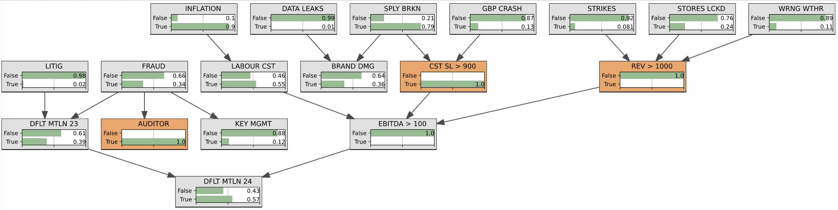
gnb.showInference(bn, evs={'REV > 1000': 0, 'CST SL > 900': 1})

In the case we observe from the new income statement that the cost of sales has increased above GBP 900mn and the revenue has fallen below GBP 1bn, we can deduce that the estimated default probability at 2 years for Matalan is now 38%, a 31% increase!
Reminder: Those numbers are not reliable, and not an investment advice.
Inference in the whole Bayes net with one more piece of evidence
gnb.showInference(bn, evs={'REV > 1000': 0, 'CST SL > 900': 1, 'AUDITOR': 1})

Let’s now suppose that the company just changed its auditors, and we were notified of it. Given the very low probability of a company changing its auditors, we may suspect something fishy is going on, i.e. the risk of accounting fraud is elevated (indeed it increases from 1% to 34%). The high fraud risk is increasing the default probability on the ‘23 Notes, which consequently increases the risk of default on the ‘24 Notes to 57% (a further increase of 50%).
Reminder: Those numbers are not reliable, and not an investment advice.