Classification of Correlation Matrices using SPDNet with Riemannian Batch Normalization
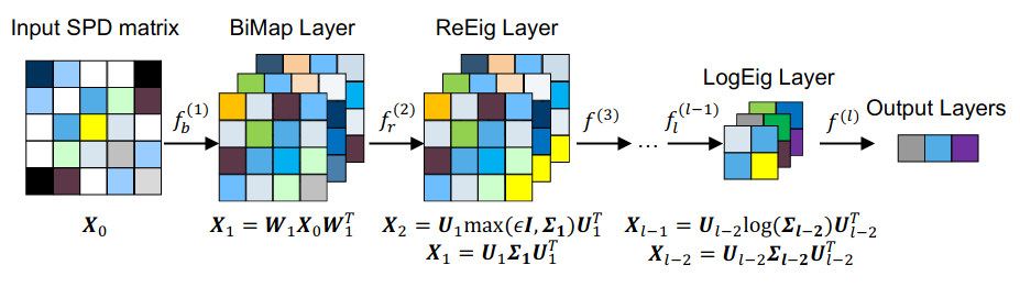 Illustration from "A Riemannian Network for SPD Matrix Learning" https://arxiv.org/pdf/1608.04233.pdf
Classification of Correlation Matrices using SPDNet with Riemannian Batch Normalization
You can find the reproducible experiment in this Colab Notebook.
In this blog, I explore the relatively recent SPDNet, and its extension: SPDNet + Riemannian Batch Normalization. They could be interesting building blocks to improve my CorrGAN/CovGAN models, and their conditional extensions.
The torchspdnet library I’m using has been developed by Olivier Schwander (a PhD-brother, i.e. same PhD supervisor: Frank Nielsen).
One of the main contribution of the associated paper is to use the Karcher flow algorithm in order to compute the Riemannian barycenter (also known as the Fréchet mean). This mean, which is the point on the Riemannian manifold of covariance matrices minimizing inertia (in terms of the associated Riemannian metric), is used to center the batch given to the neural net model.
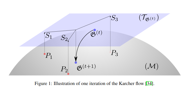 From "Riemannian batch normalization for SPD neural networks" https://arxiv.org/pdf/1909.02414.pdf (NeurIPS 2019)
TL;DR SPDNet + Riemannian Batch Normalization is quite data-efficient: The neural net provides good results with not so much data points. It could be a useful building block for a revamped CorrGAN/CovGAN.
Code and results
Load the PyTorch SPDNet library and the dataset of $80 \times 80$ correlation matrices. Such a dataset has already been described in a previous blog.
!git clone https://gitlab.lip6.fr/schwander/torchspdnet.git
%cd torchspdnet

!python setup.py install

import os, sys
sys.path.append(os.getcwd())

!wget "https://sp500-histo.s3-ap-southeast-1.amazonaws.com/CorrMats.zip"
!unzip -q CorrMats
You should be able to see 18,000 correlation matrices in your Colab drive.
%ll '/content/torchspdnet/CorrMats' | wc
18001 144002 1062903
import random

import numpy as np
import torch as th
import torch.nn as nn
from torch.utils import data
import pandas as pd
import matplotlib.pyplot as plt

import torchspdnet.nn as spdnet
from torchspdnet.optimizers import MixOptimizer
Definition of the SPDNet + RBN (optional) model.
This one is very simple, with essentially one layer, as we will work with relatively small correlation matrices and small samples:
class CorrMatsNet(nn.Module):
    def __init__(self, bn=False):
        super(__class__, self).__init__()
        dim = 80
        dim1 = 30
        classes = 3
        self._bn = bn
        self.bimap1 = spdnet.BiMap(1, 1, dim, dim1)
        if bn:
            self.batchnorm1 = spdnet.BatchNormSPD(dim1)
        self.logeig = spdnet.LogEig()
        self.linear = nn.Linear(dim1**2, classes).double()
    def forward(self, x):
        x = self.bimap1(x)
        if self._bn:
            x = self.batchnorm1(x)
        x = self.logeig(x)
        x_vec = x.view(x.shape[0], -1)
        y = self.linear(x_vec)
        return y
The whole initial dataset:
# by construction, the 3 classes have same cardinal:
# class 0: 6000 'stressed' correlation matrices
# class 1: 6000 'normal' correlation matrices
# class 2: 6000 'rally' correlation matrices
data_path = '/content/torchspdnet/CorrMats/'
for filenames in os.walk(data_path):
    names = filenames[2]
print(f'# matrices = {len(names)}')

random.Random(0).shuffle(names)
# matrices = 18000
Each correlation matrix has a label attached: ‘stressed’ or ‘normal’ or ‘rally’. This label corresponds approximately to a market regime, which was determined by the Sharpe ratio of the associated 80 stocks during the period when the matrix was estimated. More details there.
class DatasetCorrMats(data.Dataset):
    def __init__(self, path, names):
        self._path = path
        self._names = names
    def __len__(self):
        return len(self._names)
    def __getitem__(self, item):
        x = np.load(self._path + self._names[item])[None, :, :].real
        x = th.from_numpy(x).double()
        y = int(self._names[item].split('_')[3].split('.')[0])
        y = th.from_numpy(np.array(y)).long()
        return x, y
Function to train the SPDNet model, with the optional Riemannian Batch Normalization (RBN):
def train_model(train_generator, test_generator, use_rbn=True,
                batch_size=30, lr=1e-2, threshold_reeig = 1e-4, epochs=30,
                n=80, C=3):

  model = CorrMatsNet(bn=use_rbn)

  loss_fn = nn.CrossEntropyLoss()
  opti = MixOptimizer(model.parameters(),lr=lr)

  #initial validation accuracy
  loss_val, acc_val = [], []
  y_true, y_pred = [], []
  model.eval()
  for local_batch, local_labels in test_generator:
      out = model(local_batch)
      l = loss_fn(out, local_labels)
      predicted_labels=out.argmax(1)
      y_true.extend(list(local_labels.cpu().numpy()))
      y_pred.extend(list(predicted_labels.cpu().numpy()))
      acc, loss = ((predicted_labels==local_labels)
                  .cpu()
                  .numpy()
                  .sum()/out.shape[0],
                  l.cpu().data.numpy())
      loss_val.append(loss)
      acc_val.append(acc)
  acc_val = np.asarray(acc_val).mean()
  loss_val = np.asarray(loss_val).mean()
  print('Initial validation accuracy: ' + str(round(100 * acc_val, 2)) + '%')
  spdnet_acc = []
  spdnet_acc.append(acc_val)

  #training loop
  for epoch in range(epochs):

      # train one epoch
      loss_train, acc_train = [], []
      model.train()
      for local_batch, local_labels in train_generator:
          opti.zero_grad()
          out = model(local_batch)
          l = loss_fn(out, local_labels)
          acc, loss = ((out.argmax(1) == local_labels)
                      .cpu()
                      .numpy()
                      .sum()/out.shape[0],
                      l.cpu().data.numpy())
          loss_train.append(loss)
          acc_train.append(acc)
          l.backward()
          opti.step()
      acc_train = np.asarray(acc_train).mean()
      loss_train = np.asarray(loss_train).mean()

      # validation
      acc_val_list = []
      y_true, y_pred = [], []
      model.eval()
      for local_batch, local_labels in test_generator:
          out = model(local_batch)
          l = loss_fn(out, local_labels)
          predicted_labels = out.argmax(1)
          y_true.extend(list(local_labels.cpu().numpy()))
          y_pred.extend(list(predicted_labels.cpu().numpy()))
          acc, loss = ((predicted_labels == local_labels)
                      .cpu()
                      .numpy()
                      .sum()/out
                      .shape[0],
                      l.cpu().data.numpy())
          acc_val_list.append(acc)
      acc_val = np.asarray(acc_val_list).mean()

      if (epoch + 1) % 10 == 0:
        print('Val acc: ' + str(round(100 * acc_val, 2)) + '% at epoch ' +
              str(epoch + 1) + '/' + str(epochs))

      spdnet_acc.append(acc_val)

  return spdnet_acc, model
acc_results = []
std_results = []
batch_size = 32
train_sizes = [100, 200, 300, 400, 500]
for use_rbn in [True, False]:
  for train_size in train_sizes:
    print(f'Train sample size: {train_size} with RBN={use_rbn}')

    for id_class in range(3):
      class_card = len([f for f in names[:train_size]
                        if f[-5:-4] == str(id_class)])
      print(f'Class {id_class} cardinal = {class_card}')

    train_set = DatasetCorrMats(data_path, names[:train_size])
    test_set = DatasetCorrMats(data_path, names[-500:])

    train_generator = data.DataLoader(
        train_set, batch_size=batch_size, shuffle='True')
    test_generator = data.DataLoader(
        test_set, batch_size=batch_size, shuffle='False')

    test_accuracy, model = train_model(
        train_generator, test_generator, use_rbn=use_rbn)

    acc_results.append(test_accuracy)
acc_results = np.array(acc_results)
Train sample size: 100 with RBN=True
Class 0 cardinal = 37
Class 1 cardinal = 31
Class 2 cardinal = 32
Initial validation accuracy: 34.34%
Val acc: 57.58% at epoch 10/30
Val acc: 56.84% at epoch 20/30
Val acc: 57.66% at epoch 30/30
Train sample size: 200 with RBN=True
Class 0 cardinal = 70
Class 1 cardinal = 62
Class 2 cardinal = 68
Initial validation accuracy: 30.0%
Val acc: 54.84% at epoch 10/30
Val acc: 59.26% at epoch 20/30
Val acc: 58.05% at epoch 30/30
Train sample size: 300 with RBN=True
Class 0 cardinal = 106
Class 1 cardinal = 96
Class 2 cardinal = 98
Initial validation accuracy: 31.6%
Val acc: 57.03% at epoch 10/30
Val acc: 59.65% at epoch 20/30
Val acc: 58.32% at epoch 30/30
Train sample size: 400 with RBN=True
Class 0 cardinal = 144
Class 1 cardinal = 133
Class 2 cardinal = 123
Initial validation accuracy: 32.03%
Val acc: 58.75% at epoch 10/30
Val acc: 58.91% at epoch 20/30
Val acc: 58.75% at epoch 30/30
Train sample size: 500 with RBN=True
Class 0 cardinal = 170
Class 1 cardinal = 165
Class 2 cardinal = 165
Initial validation accuracy: 34.45%
Val acc: 56.45% at epoch 10/30
Val acc: 58.48% at epoch 20/30
Val acc: 58.75% at epoch 30/30
Train sample size: 100 with RBN=False
Class 0 cardinal = 37
Class 1 cardinal = 31
Class 2 cardinal = 32
Initial validation accuracy: 39.1%
Val acc: 33.91% at epoch 10/30
Val acc: 36.95% at epoch 20/30
Val acc: 33.98% at epoch 30/30
Train sample size: 200 with RBN=False
Class 0 cardinal = 70
Class 1 cardinal = 62
Class 2 cardinal = 68
Initial validation accuracy: 33.16%
Val acc: 33.95% at epoch 10/30
Val acc: 42.07% at epoch 20/30
Val acc: 46.68% at epoch 30/30
Train sample size: 300 with RBN=False
Class 0 cardinal = 106
Class 1 cardinal = 96
Class 2 cardinal = 98
Initial validation accuracy: 33.79%
Val acc: 38.63% at epoch 10/30
Val acc: 45.2% at epoch 20/30
Val acc: 53.59% at epoch 30/30
Train sample size: 400 with RBN=False
Class 0 cardinal = 144
Class 1 cardinal = 133
Class 2 cardinal = 123
Initial validation accuracy: 35.74%
Val acc: 40.04% at epoch 10/30
Val acc: 43.01% at epoch 20/30
Val acc: 52.27% at epoch 30/30
Train sample size: 500 with RBN=False
Class 0 cardinal = 170
Class 1 cardinal = 165
Class 2 cardinal = 165
Initial validation accuracy: 30.63%
Val acc: 45.98% at epoch 10/30
Val acc: 57.38% at epoch 20/30
Val acc: 59.1% at epoch 30/30
plt.figure(figsize=(18, 10))
colors = ['r', 'g', 'b', 'c', 'm', 'y', 'k']
for i, train_size in enumerate(train_sizes):
  plt.plot(acc_results[i, :], '-o', color=colors[i % len(colors)],
           label=f'train sample size = {train_size} w/ RBN')
for i, train_size in enumerate(train_sizes):
  plt.plot(acc_results[i + len(train_sizes), :], '--',
           color=colors[i % len(colors)],
           label=f'train sample size = {train_size} w/o RBN')
plt.xlabel('epochs', fontsize=16)
plt.ylabel('accuracy', fontsize=16)
plt.title('Accuracy as a function of sample size, epochs, ' +
          'and use of Riemannian batch normalization', fontsize=20)
plt.legend(fontsize=14)
plt.show()
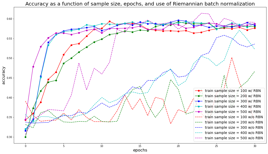
We can observe that results are more stable and accuracy converges faster with the Riemannian Batch Normalization layer: The model requires less data points and training iterations (epochs) to achieve the same results.
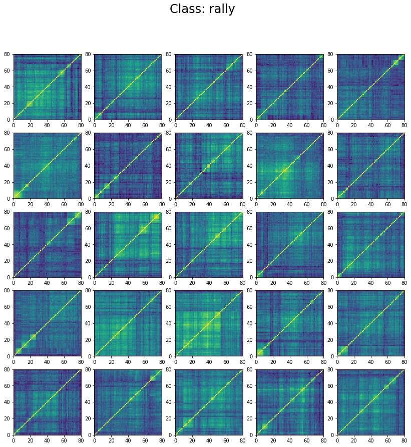
We can wonder why the model stalls at 60% accuracy only. However, if we inspect the classes in the training set we can understand why. Let’s display 25 instances of each class:
for id_class, regime in enumerate(['stressed', 'normal', 'rally']):
  plt.figure(figsize=(14, 14))
  count = 0
  for pt in train_set:
    if pt[1] == id_class:
      plt.subplot(5, 5, count + 1)
      plt.pcolormesh(pt[0][0, :, :])
      count += 1
      if count >= 25:
        break
  plt.suptitle(f'Class: {regime}', fontsize=24)
  plt.show()
We can see below that the classes are not well separated in the training set:
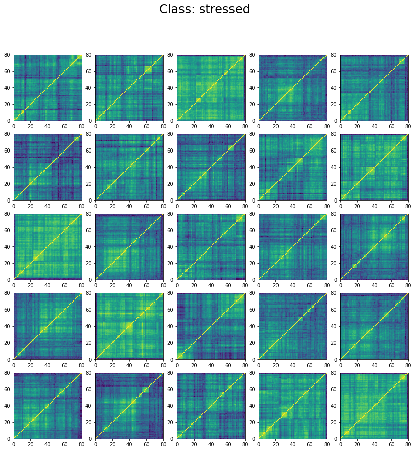
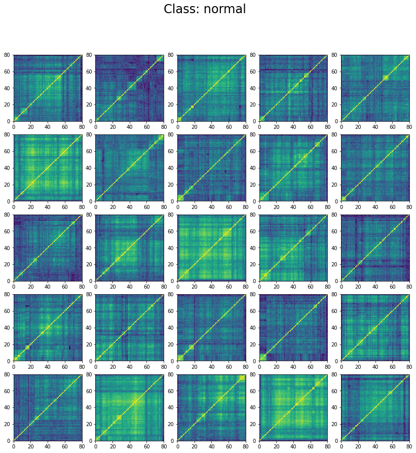
The preparation of the dataset (correlation matrix, label) was indeed quite naive (basic thresholds determined somewhat arbitrarily).
This could be improved by using
- clustering of correlation matrices (to determine first the $k$ regimes, and then associate a given correlation matrix to its closest regime),
- regime detection algorithms (e.g. HMMs), etc.
In short, many correlation matrices may be mislabeled.
Re-labeling the dataset more accurately can be future work (e.g. using the aforementioned techniques, or a trained classifier to find the suspicious (low confidence classification) data points, re-label them, and re-iterate the training/re-labeling process until some sort of fixed point).
It can also come from the fact that many correlation matrices are ‘in-between’ two regimes (e.g. normal/stress or normal/rally), and are sometimes associated to one or the other. In that case, it should correspond to low-confidence regions for the classifier.
Let’s quickly check with a classifier trained on 500 correlation matrices.
train_size = 500

train_set = DatasetCorrMats(data_path, names[:train_size])
test_set = DatasetCorrMats(data_path, names[-500:])

train_generator = data.DataLoader(
    train_set, batch_size=batch_size, shuffle='True')
test_generator = data.DataLoader(
    test_set, batch_size=batch_size, shuffle='False')

test_accuracy, model = train_model(
    train_generator, test_generator, use_rbn=True)
Initial validation accuracy: 31.05%
Val acc: 56.88% at epoch 10/30
Val acc: 57.93% at epoch 20/30
Val acc: 58.16% at epoch 30/30
Let’s predict the labels on the whole test set (500 different correlation matrices).
predictions = []
for i in range(len(test_set)):
  t = test_set[i][0].reshape(1, 1, 80, 80)
  out = model(t)
  predictions.append(out.detach().numpy()[0].tolist())
predictions = pd.DataFrame(predictions,
                           columns=['stressed', 'normal', 'rally'])
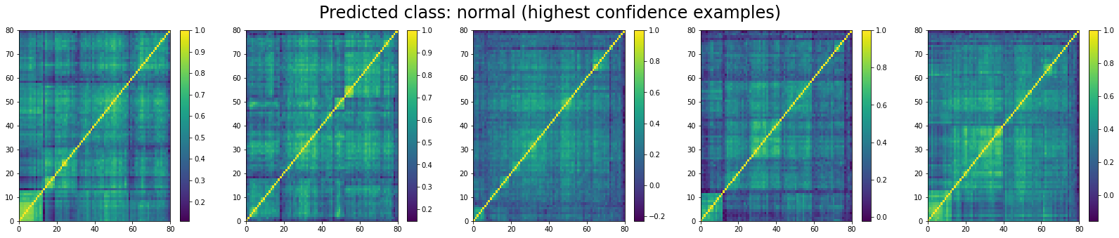
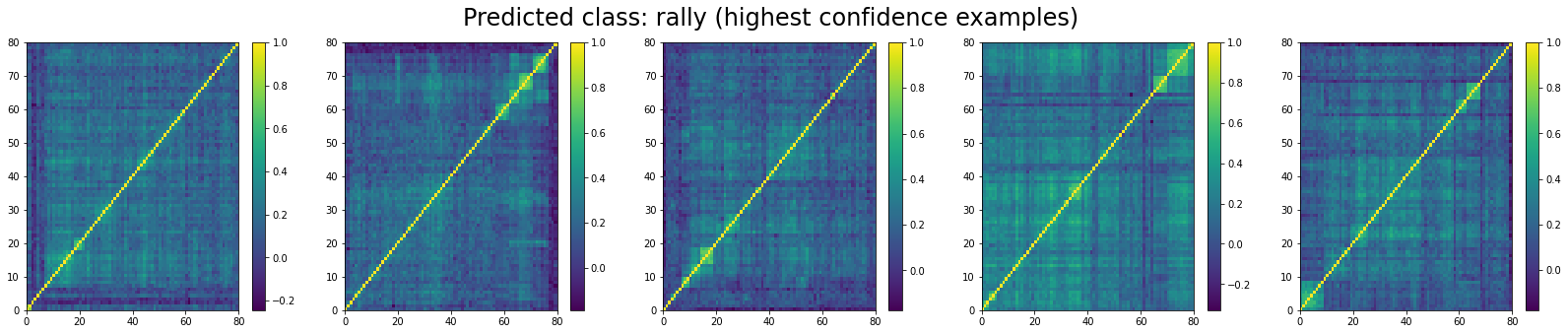
for cur_class in ['stressed', 'normal', 'rally']:
most_typical = (predictions
.sort_values(cur_class, ascending=False)
.head(5)
.index)
plt.figure(figsize=(28, 5))
for i, idx in enumerate(most_typical):
plt.subplot(1, 5, i + 1)
plt.pcolormesh(test_set[idx][0][0, :, :])
plt.colorbar()
plt.suptitle(f'Predicted class: {cur_class} (highest confidence examples)',
fontsize=24)
plt.show()
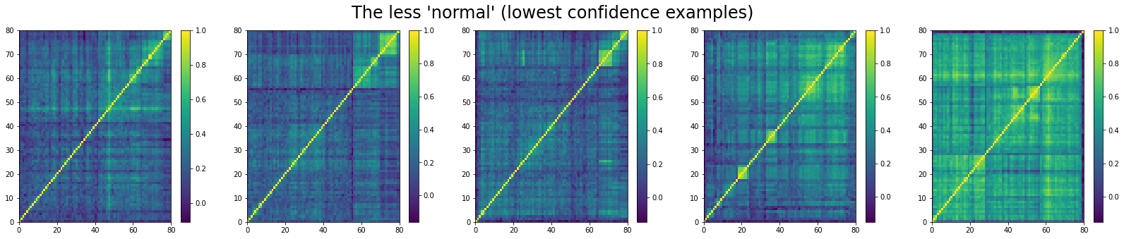
less_typical = (predictions
.sort_values(cur_class, ascending=False)
.tail(5)
.index)
plt.figure(figsize=(28, 5))
for i, idx in enumerate(less_typical):
plt.subplot(1, 5, i + 1)
plt.pcolormesh(test_set[idx][0][0, :, :])
plt.colorbar()
plt.suptitle(f"The less '{cur_class}' (lowest confidence examples)",
fontsize=24)
plt.show()
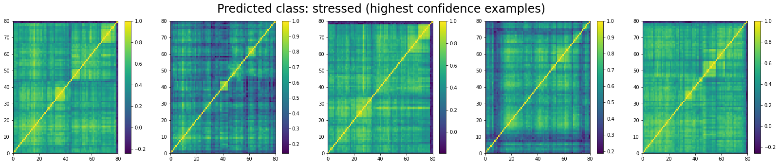
Now, let’s display the 5 correlation matrices where the classifier has the highest confidence in them being associated to a ‘stressed’ market regime:
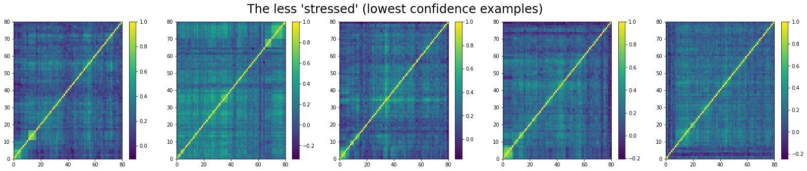
And the 5 correlation matrices which are the less likely to be associated to a ‘stressed’ market regime:
We do the same for ‘normal’ correlation matrices. The top 5:
And, the bottom 5:
For ‘rally’ correlation matrices, the top 5 looks like:
And, the bottom 5 looks like:
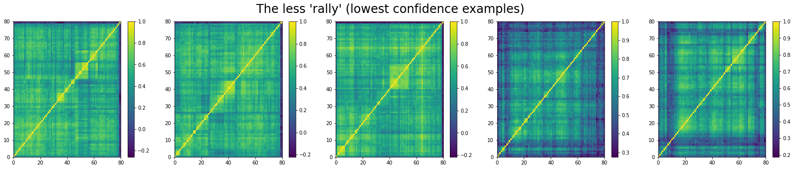
We can see that ‘stressed’ and ‘rally’ correlation matrices have a clear distinct pattern, whereas the ‘normal’ class seems to contain matrices which could be ‘stressed’ or ‘rally’.
Conclusion: It seems that using a Riemannian geometry approach in the design of the neural nets and their training leads to more data-efficient models (good results with less data). However, it’s possible that these advanced deep learning models perform on a par with more straightforward architectures such as CNNs when tons of data are available, if not worse because they are slow(er) to train… and thus they might not be able to leverage as much data as simpler neural nets. I shall try to illustrate that point in a future blog: CNN vs. SPDNet.
NB In this blog, we worked with correlation matrices whereas the SPDNet is designed for the space of covariance matrices. It’s true that any correlation matrix is a covariance matrix, so it’s fine to use this SPDNet.
However, the space of correlation matrices is not totally geodesic in the space of covariance matrices, which means that the mean of correlation matrices is not necessarily a correlation matrix but a covariance matrix.
For example, let’s consider the following 3-dimensional SPD cone:

Each $2 \times 2$ covariance matrix is represented by a point $(x, y, z)$. The blue segment $(x = z = 1)$ is the set of $2 \times 2$ correlation matrices. In green, the geodesic (using the Riemannian Fisher-Rao metric for covariances) between correlation matrix $(1, −0.75, 1)$ and correlation matrix $(1, 0.75, 1)$. The geodesic $\gamma(t)$ (and in particular the Riemannian mean $\gamma(0.5)$) is not included in the blue segment representing the correlation matrix space.
Therefore, despite SPDNet starts from correlation matrices as input, it will generate covariance matrices in downstream layers.
How can we fix that? We can renormalize at each layer using the transform $C = diag(\Sigma)^{-\frac{1}{2}} \Sigma diag(\Sigma)^{-\frac{1}{2}}$ to go from covariance matrix $\Sigma$ to correlation matrix $C$.
But, it’s not clear to me that geometrically it is the correct thing to do… any ideas?