Classification in Tones of Audio Speech

Serious, Sassy, or Sad? Teaching Machines to Read the Room (From Speech Embeddings)

📌 A politician says ‘We are fully in control of the situation’ — but their voice is trembling. Would you trust the words or the tone? Can AI detect when speech and vocal tone don’t match?

Introduction
The experiment
Research question
tl;dr
Loading the Embeddings
Understanding the Embeddings
Implications
Validating the Findings with Supervised Classification
Short vs. Long Sentences
🔍 Key Takeaways
Discrepancy Index – A Future Research Direction

N.B. This blog post serves as a pedagogical introduction to the core concepts and methodologies explored in Hamdan Al Ahbabi’s PhD research as part of his doctoral studies at Khalifa University, under my co-supervision. It is entirely non-work-related and should not be interpreted as such. Instead, its purpose is to support and complement future presentations at academic conferences.

Introduction

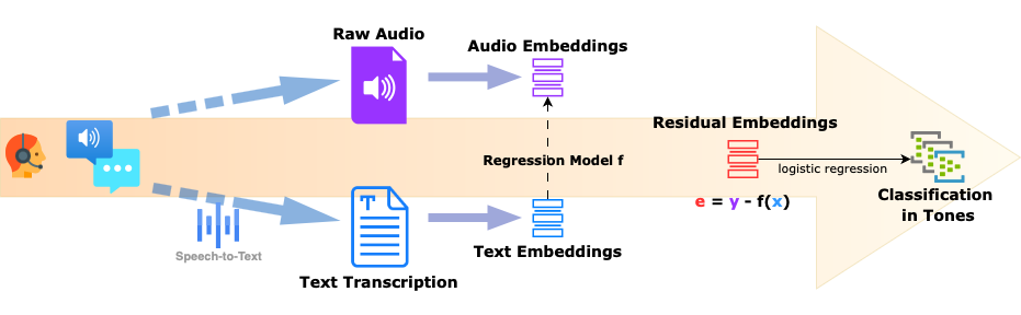
In our previous blog post, Disentangling Speech Embeddings, we introduced a simple yet effective method for removing linguistic content (what is being said) from speech embeddings. Concretely, we trained a linear model to predict raw speech embeddings from the corresponding text embeddings and used the residuals (differences) as a proxy for non-linguistic vocal features. We demonstrated that the resulting “residual” embeddings retained enough vocal cue information to cluster sentences by speaker identity rather than semantic content — suggesting that these embeddings preserve vocal tone and style independently of the words spoken.

Now, we take this idea one step further. This time, we explore whether these residual embeddings can help classify how something is said—focusing on vocal tone and speaking style.

The experiment

We use a single speaker (a female, US English voice - Natalie from murf.ai) and have her deliver different sentences across a variety of tones and styles. The sentences range from neutral business jargon to casual, sentiment-laden phrases (both positive and negative). The 12 distinct tones/styles tested include: Sorrowful, Inspirational, Terrified, Furious, Newscast Casual, Conversational, Angry, Sad, Meditative, Newscast Formal, Narration, and Promo.

Research question

👉 Is it easier to classify speech into one of these 12 tones/styles using the original wav2vec2 audio embeddings, or does the “residual” version (where content has been removed) provide a cleaner signal for tone classification?

tl;dr

✅ Both linear and non-linear models perform better using the residual embeddings than the raw audio ones, where the actual spoken content appears to confuse the model.

✅ Linear and non-linear classifiers perform similarly, suggesting that the relevant information (tone/style) is well-captured in a way that can be extracted with simple linear methods.

✅ Shorter sentences provide fewer vocal cues, making tone classification harder. Residual embeddings help the most in these cases by removing content interference.

✅ With longer sentences, tone information is naturally stronger, reducing the need for content filtering—though residual embeddings still offer a slight edge.

✅ This supports the idea that removing linguistic content enhances models’ ability to focus on paralinguistic features (tone, style, speaker characteristics).

Loading the Embeddings

Let’s start by loading the data (sentences and embeddings).

import os
import numpy as np
import pandas as pd
import matplotlib.pyplot as plt
import seaborn as sns
from sklearn.linear_model import Ridge, LogisticRegression
from sklearn.ensemble import RandomForestClassifier
from sklearn.metrics import (
    accuracy_score, f1_score, roc_auc_score, confusion_matrix)
from sklearn.model_selection import train_test_split
from sklearn.decomposition import PCA
from sklearn.manifold import TSNE


styles = [
    "Sorrowful", "Inspirational", "Terrified",
    "Furious", "Newscast Casual", "Conversational",
    "Angry", "Sad", "Meditative",
    "Newscast Formal", "Narration", "Promo",
]


sentences = pd.read_parquet("earnings_calls_sentences.parquet")
positive_sentences = pd.read_parquet("positive_sentences.parquet")
negative_sentences = pd.read_parquet("negative_sentences.parquet")

display(sentences.sample(5))
display(positive_sentences.sample(5))
display(negative_sentences.sample(5))

	sentence
5	For the next 100 years to come, we will contin...
36	It's not just that we recruit the best or that...
13	You see the overseas sales ratio of the in-hou...
46	Compared to the IOCs over the last five years,...
31	Not just profitable growth for ExxonMobil, but...

	sentence
25	The resilience and optimism you maintain in th...
3	That meal was incredibly delicious.
10	Your kindness and generosity are truly inspiring.
18	Everything is going so well—I feel incredibly ...
4	I'm so proud of you for achieving your goal!

	sentence
15	I couldn't be more frustrated with how things ...
8	You are the most unreliable person I've ever met.
37	It is disheartening to see that despite having...
5	You always find a way to make things worse.
1	I absolutely hate dealing with this kind of si...

df_audio_emb = pd.read_parquet("wav2vec2_audio_embeddings.parquet")
df_text_emb = pd.read_parquet("dataframe_text_embeddings.parquet")

# Convert DataFrames to NumPy arrays
X = df_text_emb.values    # shape: (n_samples, 1536)
Y = df_audio_emb.values   # shape: (n_samples, 768)

print("Text embeddings shape:", X.shape)
print("Audio embeddings shape:", Y.shape)

Text embeddings shape: (1584, 1536)
Audio embeddings shape: (1584, 768)

# Train Ridge regression model
def train_ridge_regression(X, Y, alpha=1.0):
    model = Ridge(alpha=alpha)
    model.fit(X, Y)
    return model

model = train_ridge_regression(X, Y)

# Compute residual embeddings
Y_pred = model.predict(X)
E = Y - Y_pred

df_residual_emb = pd.DataFrame(E, index=df_audio_emb.index)

df_residual_emb

	0	1	2	3	4	5	6	7	8	9	...	758	759	760	761	762	763	764	765	766	767
sent_speaker
embeddings_downloaded_audio_00_Angry.npy	0.000547	-0.005123	0.033253	-0.038299	0.013721	-0.038447	0.007130	0.023777	0.000756	-0.018350	...	-0.011541	-0.012827	0.026055	-0.032220	-0.038547	0.006204	-0.010762	0.002884	-0.038804	0.044158
embeddings_downloaded_audio_00_Conversational.npy	-0.012998	0.003234	0.010352	-0.004429	0.019514	-0.000994	0.014857	0.005752	-0.004121	-0.029278	...	-0.032924	0.002646	0.021952	0.001924	-0.037578	-0.013107	-0.020910	-0.005894	0.017660	-0.035358
embeddings_downloaded_audio_00_Furious.npy	-0.066253	0.015863	-0.018699	0.040799	-0.021040	0.018685	0.038205	-0.000754	0.012815	-0.008809	...	0.003965	0.008530	0.002404	-0.032704	0.055339	-0.023414	-0.019636	0.023885	-0.000745	-0.023359
embeddings_downloaded_audio_00_Inspirational.npy	-0.002424	-0.028308	0.000459	0.002153	-0.007286	0.022152	-0.025893	-0.025777	-0.058059	-0.007379	...	0.016637	-0.011735	0.017605	0.017890	0.033506	0.005326	-0.003464	-0.004350	-0.007208	0.026986
embeddings_downloaded_audio_00_Meditative.npy	0.001378	-0.011582	0.036844	-0.042164	-0.036087	0.010559	-0.005657	0.025860	-0.070218	0.003857	...	0.046636	0.004565	0.011343	-0.003232	-0.006497	-0.026536	0.002865	-0.012032	-0.005313	0.042849
...	...	...	...	...	...	...	...	...	...	...	...	...	...	...	...	...	...	...	...	...	...
embeddings_positive_text_downloaded_audio_39_Newscast Formal.npy	-0.010689	-0.001865	-0.040611	0.009453	0.047540	-0.027685	0.015540	0.012837	0.010790	0.011269	...	-0.015807	-0.010005	-0.005689	-0.000988	-0.033687	0.001929	0.008778	-0.015480	-0.008912	-0.012508
embeddings_positive_text_downloaded_audio_39_Promo.npy	-0.035135	0.026699	-0.025716	-0.008928	0.055495	0.066652	0.038595	-0.007269	-0.032083	-0.002548	...	0.044913	0.003458	0.005861	-0.050246	0.004993	0.000369	0.010904	-0.010641	-0.021717	-0.054168
embeddings_positive_text_downloaded_audio_39_Sad.npy	0.019876	0.014143	-0.087296	0.017254	0.075202	-0.049448	-0.006937	-0.039578	0.067603	-0.001711	...	-0.036482	-0.010577	-0.000425	0.051968	-0.067635	0.016389	-0.007544	-0.042562	0.022262	-0.001306
embeddings_positive_text_downloaded_audio_39_Sorrowful.npy	0.021177	-0.034878	-0.025202	0.025799	-0.004771	-0.026035	-0.018924	-0.022863	0.038629	-0.001309	...	-0.024871	0.010005	0.003231	0.040676	0.012732	-0.019660	0.016285	-0.011352	0.044231	0.067834
embeddings_positive_text_downloaded_audio_39_Terrified.npy	0.019007	-0.010457	0.005947	0.026304	-0.048532	0.004886	-0.005772	-0.014250	0.044395	0.002009	...	0.006794	0.008677	0.002136	0.020690	0.000381	-0.016183	0.008968	0.016245	0.035921	0.059694

1584 rows × 768 columns

Understanding the Embeddings

To begin, we visualize the embeddings by projecting them into a 2D space using standard dimensionality reduction techniques like PCA and t-SNE. This allows us to explore whether any clear structure emerges in these representations.

X_text = df_text_emb.values
X_audio = df_audio_emb.values
X_resid = df_residual_emb.values

# Extract labels: assuming styles are encoded in filenames
labels = pd.Series([elem.split('_')[-1].split('.npy')[0]
                    for elem in df_audio_emb.index])

def plot_pca_tsne(X, labels, title_prefix):
    """
    Apply PCA and t-SNE to reduce dimensions and visualize embeddings.
    """
    # Convert labels to categorical numeric values
    label_values, label_mapping = pd.factorize(labels)

    # Apply PCA
    pca = PCA(n_components=2)
    X_pca = pca.fit_transform(X)

    # Apply t-SNE
    tsne = TSNE(n_components=2, perplexity=5, random_state=42)
    X_tsne = tsne.fit_transform(X)

    fig, axes = plt.subplots(1, 2, figsize=(14, 6))

    # PCA Plot
    scatter = axes[0].scatter(
        X_pca[:, 0], X_pca[:, 1],
        c=label_values, cmap="tab20", alpha=0.7)
    axes[0].set_title(f"{title_prefix} - PCA Projection")
    axes[0].set_xlabel("PC1")
    axes[0].set_ylabel("PC2")

    # t-SNE Plot
    scatter = axes[1].scatter(
        X_tsne[:, 0], X_tsne[:, 1],
        c=label_values, cmap="tab20", alpha=0.7)
    axes[1].set_title(f"{title_prefix} - t-SNE Projection")
    axes[1].set_xlabel("t-SNE Dim 1")
    axes[1].set_ylabel("t-SNE Dim 2")

    # Add legend for the unique labels
    legend_labels = {i: label for i, label in enumerate(label_mapping)}
    handles = scatter.legend_elements()[0]
    labels_list = [legend_labels[i] for i in range(len(handles))]
    axes[1].legend(handles, labels_list,
                   loc="best", fontsize="small", title="Styles")

    plt.show()


    
# Run PCA & t-SNE for Text Embeddings
content_labels = pd.Series(
    ["business"] * 52 * 12 + ["negative"] * 40 * 12 + ["positive"] * 40 * 12)
plot_pca_tsne(X_text, content_labels, "Text Embeddings")

# Run PCA & t-SNE for Audio Embeddings
plot_pca_tsne(X_audio, labels, "Audio Embeddings")

# Run PCA & t-SNE for Residual Embeddings
plot_pca_tsne(X_resid, labels, "Residual Embeddings")

Text Embeddings 2D Projections

Audio Embeddings 2D Projections

Residual Embeddings 2D Projections

These visualizations confirm that residual embeddings provide clearer clustering by tone, reinforcing their usefulness in capturing vocal style.

In more details:

Text Embeddings

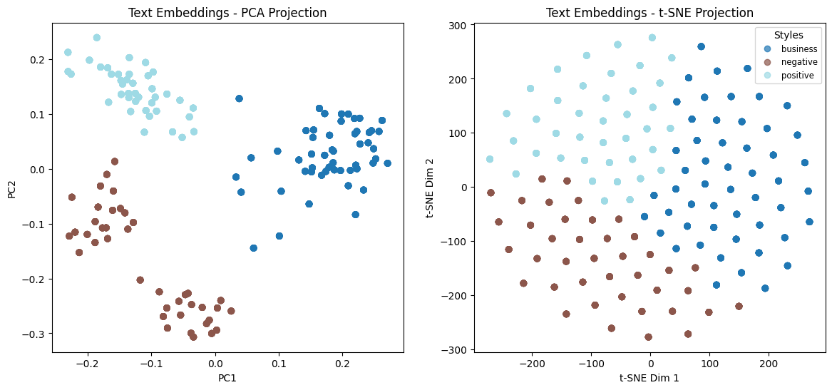
The first row displays the text embeddings projected onto a two-dimensional space using PCA (left) and t-SNE (right). Since these embeddings represent only the textual content and not the way sentences are spoken, the different tone/style labels do not appear distinct in the PCA projection. Instead, we only observe clusters corresponding to:

Business-related sentences (52 samples)
Positive sentiment sentences (40 samples)
Negative sentiment sentences (40 samples)

This indicates that text embeddings primarily encode content (and sentiment).

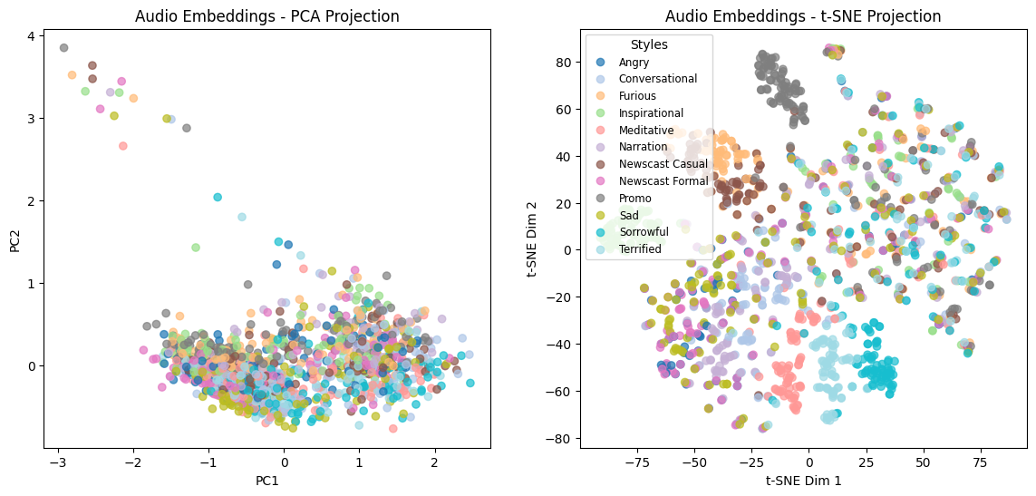
Audio Embeddings

For the raw audio embeddings, the PCA projection (center-left) does not exhibit clear structure. While a handful of outliers are present, the majority of the data points are densely packed without clear separation. This suggests that in their raw form, audio embeddings mix linguistic content and vocal tone/style, making them difficult to disentangle.

However, when applying t-SNE (center-right), we start to observe some degree of clustering by tone/style. Notably:

The “Promo” (grey) and “Furious” (orange) styles form noticeable clusters.
Other styles remain partially mixed, indicating that raw audio embeddings do encode tone information but not in a way that is easily separable.

These findings reinforce the idea that raw speech embeddings contain a blend of both linguistic and speaker-specific information, making it challenging to extract tone/style characteristics directly.

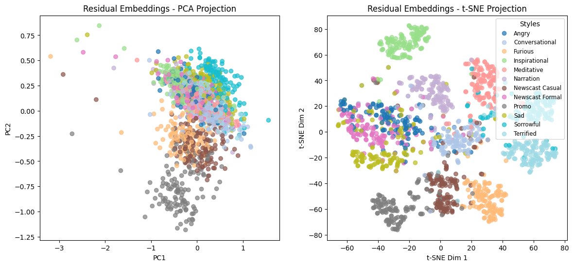
Residual Embeddings

The residual embeddings, which remove linguistic content using the elementary method presented in Disentangling Speech Embeddings, exhibit a much stronger clustering structure:

PCA projection (bottom-left) shows better-defined clusters (e.g., blue, orange, brown, grey) compared to raw audio embeddings, although the separation is not perfect.
t-SNE projection (bottom-right) reveals a remarkably clear separation of the 12 tones/styles. Unlike raw audio embeddings, the residual embeddings distinctly group sentences by how they are spoken rather than what is being said.

This result strongly suggests that removing linguistic content leaves behind a representation that is highly predictive of tone and style. In other words:

Text embeddings capture only the content of speech (what is being said).
Residual embeddings predominantly encode vocal tone/style (how it is being said).
Raw audio embeddings contain a mixture of both, making classification more difficult.

Implications

If the goal is tone/style classification, residual embeddings should be used instead of raw audio embeddings.
Residual embeddings cluster strongly by style, meaning even simple models (e.g., logistic regression) should be able to classify tone effectively.
This experiment confirms that an elementary linear disentanglement technique successfully separates tone and linguistic content in speech embeddings.

Validating the Findings with Supervised Classification

So far, our unsupervised analysis has shown that residual embeddings exhibit clearer clustering by tone/style compared to raw audio embeddings. But how well does this separation translate to practical classification performance?

To test this, we move to a supervised classification approach:

🔹 Objective: Train a classifier to predict tone/style from speech embeddings and compare performance across different representations (audio vs. residual).

🔹 Hypothesis: If residual embeddings truly capture tone/style better than raw audio embeddings, a simple classifier should achieve higher accuracy on residuals than on raw audio embeddings.

🔹 Experiment:

Train a logistic regression model and a random forest classifier on both raw audio and residual embeddings.
Compare accuracy, F1-score, and AUC-ROC across models and representations.
Evaluate whether removing linguistic content improves the model’s ability to focus on tone and style.

Let’s dive into the code and results:

# Function to train, evaluate, and return results
def evaluate_model(X, y, model, model_name):
    """Trains a model, evaluates performance, and returns metrics."""
    X_train, X_test, y_train, y_test = train_test_split(
        X, y, test_size=0.2, random_state=42)
    
    # Train model
    model.fit(X_train, y_train)
    
    # Predict
    y_pred = model.predict(X_test)
    y_proba = (
        model.predict_proba(X_test)
        if hasattr(model, "predict_proba") else None
    )
    
    # Compute Metrics
    acc = accuracy_score(y_test, y_pred)
    f1 = f1_score(y_test, y_pred, average="weighted")
    roc_auc = (
        roc_auc_score(y_test, y_proba, multi_class="ovr")
        if y_proba is not None else None
    )

    y_pred = model.predict(X)
    conf_matrix = confusion_matrix(y, y_pred)
    
    return {"Model": model_name,
            "Accuracy": acc,
            "F1 Score": f1,
            "AUC-ROC": roc_auc,
            "Confusion Matrix": conf_matrix}


# Function to display confusion matrix
def plot_confusion_matrix(conf_matrix, title):
    """Plots a confusion matrix with heatmap."""
    plt.figure(figsize=(6, 5))
    sns.heatmap(conf_matrix, annot=True, fmt="d", cmap="Blues")
    plt.xlabel("Predicted Label")
    plt.ylabel("True Label")
    plt.title(title)
    plt.show()

# Prepare data for classification tasks
def prepare_classification_data(
    df_audio_emb, df_residual_emb, df_text_emb, use_case="business"):
    if use_case == "business":
        index = (
            ~(df_audio_emb.index.str.contains("positive")) &
            ~(df_audio_emb.index.str.contains("negative")))
    elif use_case == "sentimental_text":
        index = (
            (df_audio_emb.index.str.contains("positive")) |
            (df_audio_emb.index.str.contains("negative")))
    elif use_case == "short_text":
        mask = (
            df_audio_emb.index.str.extract(r'_(\d+)_')[0]
            .astype(float)
            .between(0, 19)
        )
        mask.index = df_audio_emb.index
        index = (
            (df_audio_emb.index.str.contains("positive") |
             df_audio_emb.index.str.contains("negative")) &
            mask
        ).tolist()
    elif use_case == "long_text":
        mask = (
            df_audio_emb.index.str.extract(r'_(\d+)_')[0]
            .astype(float)
            .between(20, 39)
        )
        mask.index = df_audio_emb.index
        index = (
            (df_audio_emb.index.str.contains("positive") |
             df_audio_emb.index.str.contains("negative")) &
            mask
        ).tolist()       
    
    X_audio = df_audio_emb[index]
    y_audio = [elem.split('_')[-1].split('.npy')[0]
               for elem in X_audio.index]
    
    X_resid = df_residual_emb[index]
    y_resid = [elem.split('_')[-1].split('.npy')[0]
               for elem in X_resid.index]
    
    X_text = df_text_emb[index]
    y_text = y_audio
    
    return (X_audio, y_audio,
            X_resid, y_resid,
            X_text, y_text)

X_audio, y_audio, X_resid, y_resid, X_text, y_text = (
    prepare_classification_data(
        df_audio_emb, df_residual_emb, df_text_emb,
        use_case="business"))


# Convert labels to numerical format
unique_labels = sorted(set(y_audio))
label_mapping = {label: idx for idx, label in enumerate(unique_labels)}
y_audio = np.array([label_mapping[label] for label in y_audio])
y_resid = np.array([label_mapping[label] for label in y_resid])
y_text  = np.array([label_mapping[label] for label in y_text])

# Convert DataFrames to numpy arrays
X_audio = X_audio.to_numpy()
X_resid = X_resid.to_numpy()
X_text  = X_text.to_numpy()

# Define models
log_reg = LogisticRegression(max_iter=1000, random_state=42)
random_forest = RandomForestClassifier(n_estimators=100, random_state=42)

# Evaluate models
results = []
results.append(
    evaluate_model(X_text, y_text, log_reg, "Logistic Regression (X_text)"))
results.append(
    evaluate_model(X_audio, y_audio, log_reg, "Logistic Regression (X_audio)"))
results.append(
    evaluate_model(X_resid, y_resid, log_reg, "Logistic Regression (X_resid)"))
results.append(
    evaluate_model(X_text, y_text, random_forest, "Random Forest (X_text)"))
results.append(
    evaluate_model(X_audio, y_audio, random_forest, "Random Forest (X_audio)"))
results.append(
    evaluate_model(X_resid, y_resid, random_forest, "Random Forest (X_resid)"))

# Convert results to DataFrame
results_df = pd.DataFrame(results).drop(columns=["Confusion Matrix"])

print("\nClassification Results:")
display(results_df)

Classification Results:

	Model	Accuracy	F1 Score	AUC-ROC
0	Logistic Regression (X_text)	0.000	0.000000	0.096726
1	Logistic Regression (X_audio)	0.888	0.889941	0.990831
2	Logistic Regression (X_resid)	0.944	0.944745	0.997317
3	Random Forest (X_text)	0.000	0.000000	0.095351
4	Random Forest (X_audio)	0.800	0.797580	0.972571
5	Random Forest (X_resid)	0.920	0.919786	0.996321

As anticipated, text embeddings do not capture tone or style information, as they solely encode linguistic content. We included them in the experiment as a control to validate this assumption, and the results confirm that tone cannot be recovered from text embeddings alone. This is clearly reflected in the classification performance shown in the bar plot below:

# Plot classification results
plt.figure(figsize=(10, 5))
results_df.set_index("Model").plot(kind="bar", figsize=(10, 5))
plt.title("Classification Performance Comparison", fontsize=14)
plt.ylabel("Score", fontsize=12)
plt.xticks(rotation=45, fontsize=10)
plt.yticks(fontsize=10)
plt.legend(loc="lower right", fontsize=10)
plt.grid(True, linestyle="--", linewidth=0.5, alpha=0.7)
plt.show()

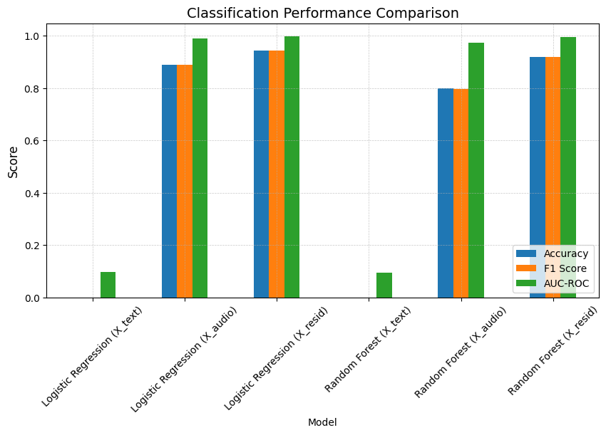
Classification Performance Comparison between Models and Embeddings

Remark: Even with simple models like logistic regression, residual embeddings achieved over 94% accuracy. This suggests that tone information is not only well-preserved but also highly predictable once linguistic content is removed. In contrast, raw audio embeddings performed worse, likely because they mix content with tone.

X_audio, y_audio, X_resid, y_resid, X_text, y_text = (
    prepare_classification_data(
        df_audio_emb, df_residual_emb, df_text_emb,
        use_case="sentimental_text"))


# Convert labels to numerical format
unique_labels = sorted(set(y_audio))
label_mapping = {label: idx for idx, label in enumerate(unique_labels)}
y_audio = np.array([label_mapping[label] for label in y_audio])
y_resid = np.array([label_mapping[label] for label in y_resid])
y_text  = np.array([label_mapping[label] for label in y_text])

# Convert DataFrames to numpy arrays
X_audio = X_audio.to_numpy()
X_resid = X_resid.to_numpy()
X_text  = X_text.to_numpy()

# Define models
log_reg = LogisticRegression(max_iter=1000, random_state=42)
random_forest = RandomForestClassifier(n_estimators=100, random_state=42)

# Evaluate models
results = []
results.append(
    evaluate_model(X_text, y_text, log_reg, "Logistic Regression (X_text)"))
results.append(
    evaluate_model(X_audio, y_audio, log_reg, "Logistic Regression (X_audio)"))
results.append(
    evaluate_model(X_resid, y_resid, log_reg, "Logistic Regression (X_resid)"))
results.append(
    evaluate_model(X_text, y_text, random_forest, "Random Forest (X_text)"))
results.append(
    evaluate_model(X_audio, y_audio, random_forest, "Random Forest (X_audio)"))
results.append(
    evaluate_model(X_resid, y_resid, random_forest, "Random Forest (X_resid)"))


# Convert results to DataFrame
results_df = pd.DataFrame(results).drop(columns=["Confusion Matrix"])

print("\nClassification Results:")
display(results_df)

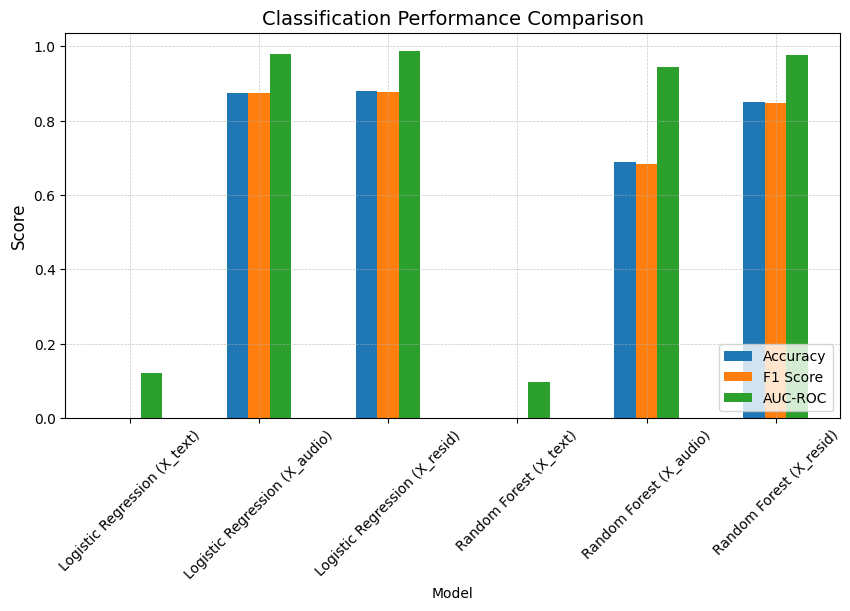
Classification Results:

	Model	Accuracy	F1 Score	AUC-ROC
0	Logistic Regression (X_text)	0.000000	0.000000	0.120661
1	Logistic Regression (X_audio)	0.875000	0.873449	0.978296
2	Logistic Regression (X_resid)	0.880208	0.878072	0.986610
3	Random Forest (X_text)	0.000000	0.000000	0.097720
4	Random Forest (X_audio)	0.687500	0.682460	0.943511
5	Random Forest (X_resid)	0.848958	0.846386	0.975307

Logistic Regression performs surprisingly well on raw audio embeddings, likely because some tone information is already linearly separable, as suggested by the earlier 2D projections. However, Random Forests show a much stronger improvement with residual embeddings, benefiting from the removal of linguistic content. By eliminating this noise, residual embeddings provide a cleaner representation of paralinguistic features, making them more suitable for decision-tree-based learning.

# Plot classification results
plt.figure(figsize=(10, 5))
results_df.set_index("Model").plot(kind="bar", figsize=(10, 5))
plt.title("Classification Performance Comparison", fontsize=14)
plt.ylabel("Score", fontsize=12)
plt.xticks(rotation=45, fontsize=10)
plt.yticks(fontsize=10)
plt.legend(loc="lower right", fontsize=10)
plt.grid(True, linestyle="--", linewidth=0.5, alpha=0.7)
plt.show()

Classification Performance Comparison between Models and Embeddings

Note: Before expanding the dataset with longer sentences, we initially ran this experiment using only 20 short positive and 20 short negative sentences. In that setup, logistic regression on raw audio embeddings achieved 0.71 accuracy, while residual embeddings improved performance to 0.82. This suggests that for shorter sentences, where vocal cues are more limited or entangled with linguistic content, residual embeddings provide a clearer benefit. By stripping away the linguistic information, they make it easier for the model to focus on paralinguistic features, leading to a more pronounced lift in classification accuracy.

This motivated us to examine whether longer, more expressive sentences improve classification performance overall and to assess whether the advantage of residual embeddings over raw audio embeddings diminishes as more vocal cues become available.

Short vs. Long Sentences

To explore this, we compare model performance on short versus long sentences, starting with the short sentence case.

The short sentences case:

X_audio, y_audio, X_resid, y_resid, X_text, y_text = (
    prepare_classification_data(
        df_audio_emb, df_residual_emb, df_text_emb,
        use_case="short_text"))


# Convert labels to numerical format
unique_labels = sorted(set(y_audio))
label_mapping = {label: idx for idx, label in enumerate(unique_labels)}
y_audio = np.array([label_mapping[label] for label in y_audio])
y_resid = np.array([label_mapping[label] for label in y_resid])
y_text  = np.array([label_mapping[label] for label in y_text])

# Convert DataFrames to numpy arrays
X_audio = X_audio.to_numpy()
X_resid = X_resid.to_numpy()
X_text  = X_text.to_numpy()

# Define models
log_reg = LogisticRegression(max_iter=1000, random_state=42)
random_forest = RandomForestClassifier(n_estimators=100, random_state=42)

# Evaluate models
results = []
results.append(
    evaluate_model(X_text, y_text, log_reg, "Logistic Regression (X_text)"))
results.append(
    evaluate_model(X_audio, y_audio, log_reg, "Logistic Regression (X_audio)"))
results.append(
    evaluate_model(X_resid, y_resid, log_reg, "Logistic Regression (X_resid)"))
results.append(
    evaluate_model(X_text, y_text, random_forest, "Random Forest (X_text)"))
results.append(
    evaluate_model(X_audio, y_audio, random_forest, "Random Forest (X_audio)"))
results.append(
    evaluate_model(X_resid, y_resid, random_forest, "Random Forest (X_resid)"))


# Convert results to DataFrame
results_df = pd.DataFrame(results).drop(columns=["Confusion Matrix"])

print("\nClassification Results:")
display(results_df)

# Plot classification results
plt.figure(figsize=(10, 5))
results_df.set_index("Model").plot(kind="bar", figsize=(10, 5))
plt.title("Classification Performance Comparison", fontsize=14)
plt.ylabel("Score", fontsize=12)
plt.xticks(rotation=45, fontsize=10)
plt.yticks(fontsize=10)
plt.legend(loc="lower right", fontsize=10)
plt.grid(True, linestyle="--", linewidth=0.5, alpha=0.7)
plt.show()

Classification Results:

	Model	Accuracy	F1 Score	AUC-ROC
0	Logistic Regression (X_text)	0.000000	0.000000	0.121146
1	Logistic Regression (X_audio)	0.708333	0.700649	0.936023
2	Logistic Regression (X_resid)	0.822917	0.817159	0.978280
3	Random Forest (X_text)	0.000000	0.000000	0.093249
4	Random Forest (X_audio)	0.552083	0.533623	0.847435
5	Random Forest (X_resid)	0.697917	0.685180	0.947323

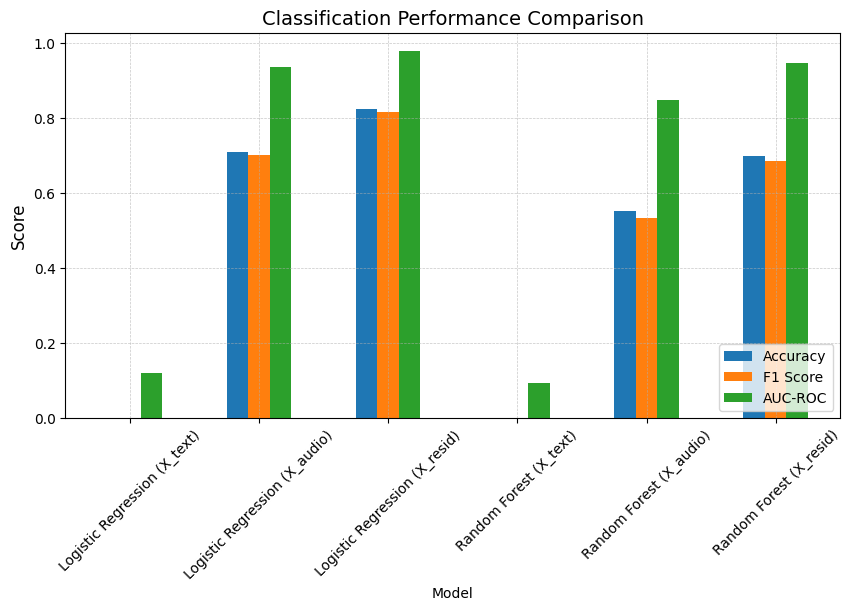
Classification Performance Comparison between Models and Embeddings

The long sentences case:

We now turn to longer sentences, where more vocal cues are naturally present.

X_audio, y_audio, X_resid, y_resid, X_text, y_text = (
    prepare_classification_data(
        df_audio_emb, df_residual_emb, df_text_emb,
        use_case="long_text"))


# Convert labels to numerical format
unique_labels = sorted(set(y_audio))
label_mapping = {label: idx for idx, label in enumerate(unique_labels)}
y_audio = np.array([label_mapping[label] for label in y_audio])
y_resid = np.array([label_mapping[label] for label in y_resid])
y_text  = np.array([label_mapping[label] for label in y_text])

# Convert DataFrames to numpy arrays
X_audio = X_audio.to_numpy()
X_resid = X_resid.to_numpy()
X_text  = X_text.to_numpy()

# Define models
log_reg = LogisticRegression(max_iter=1000, random_state=42)
random_forest = RandomForestClassifier(n_estimators=100, random_state=42)

# Evaluate models
results = []
results.append(
    evaluate_model(X_text, y_text, log_reg, "Logistic Regression (X_text)"))
results.append(
    evaluate_model(X_audio, y_audio, log_reg, "Logistic Regression (X_audio)"))
results.append(
    evaluate_model(X_resid, y_resid, log_reg, "Logistic Regression (X_resid)"))
results.append(
    evaluate_model(X_text, y_text, random_forest, "Random Forest (X_text)"))
results.append(
    evaluate_model(X_audio, y_audio, random_forest, "Random Forest (X_audio)"))
results.append(
    evaluate_model(X_resid, y_resid, random_forest, "Random Forest (X_resid)"))


# Convert results to DataFrame
results_df = pd.DataFrame(results).drop(columns=["Confusion Matrix"])

print("\nClassification Results:")
display(results_df)

# Plot classification results
plt.figure(figsize=(10, 5))
results_df.set_index("Model").plot(kind="bar", figsize=(10, 5))
plt.title("Classification Performance Comparison", fontsize=14)
plt.ylabel("Score", fontsize=12)
plt.xticks(rotation=45, fontsize=10)
plt.yticks(fontsize=10)
plt.legend(loc="lower right", fontsize=10)
plt.grid(True, linestyle="--", linewidth=0.5, alpha=0.7)
plt.show()

Classification Results:

	Model	Accuracy	F1 Score	AUC-ROC
0	Logistic Regression (X_text)	0.000000	0.000000	0.110647
1	Logistic Regression (X_audio)	0.979167	0.979601	0.996384
2	Logistic Regression (X_resid)	0.989583	0.989279	0.999267
3	Random Forest (X_text)	0.000000	0.000000	0.097023
4	Random Forest (X_audio)	0.895833	0.904243	0.989440
5	Random Forest (X_resid)	0.989583	0.989279	0.999817

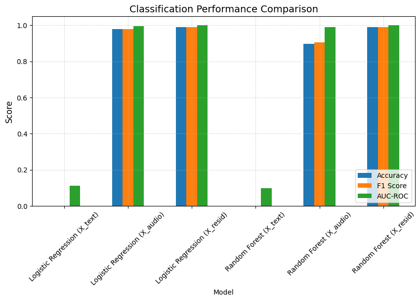
Classification Performance Comparison between Models and Embeddings

This last experiment highlights an important distinction:

Short sentences provide fewer vocal cues, making it harder for models to distinguish tone from linguistic content. In raw audio embeddings, tone information is often entangled with what is being said, making classification more difficult. This is where residual embeddings provide a significant advantage, as they strip away content-related noise and preserve only vocal tone and style.
Long sentences, on the other hand, naturally contain more vocal evidence of tone, making classification easier across all models—even when using raw audio embeddings. With longer utterances, the additional speech data allows tone to emerge more distinctly, reducing the need for content filtering. Consequently, while residual embeddings still perform best, the gap between raw and residual embeddings becomes less pronounced.

In summary, residual embeddings are most beneficial when tone cues are sparse or ambiguous, such as in short speech segments. When ample vocal evidence is available (as in longer utterances), models can more easily capture tone directly from raw embeddings, making content removal less critical.

🔍 Key Takeaways

✅ Residual embeddings cluster clearly by tone, unlike raw audio embeddings, making them a more effective representation of vocal style.

✅ Removing linguistic content enhances classification accuracy, particularly in cases where tone is subtle or mixed with content.

✅ Even simple models perform well on residual embeddings, proving that the extracted paralinguistic features are well-structured and easy to classify.

✅ Residual embeddings are especially beneficial for short sentences, where tone cues are limited and harder to separate from content in raw audio embeddings.

✅ With longer sentences, tone information becomes more pronounced in raw audio embeddings, naturally improving classification performance across the board and reducing the gap between raw and residual embeddings.

✅ Residual embeddings provide the greatest advantage when tone evidence is sparse or ambiguous, reinforcing their usefulness in analyzing brief speech segments or detecting subtle vocal cues.

Discrepancy Index – A Future Research Direction

So far, we’ve demonstrated that residual embeddings are more effective at capturing tone and style, while text embeddings reflect semantic content. But what happens when textual sentiment and vocal tone don’t align?

This opens up an exciting research question: Could we quantify such discrepancies to detect sarcasm, persuasion, or even deception?

💡 The idea:

We propose a Discrepancy Index, a metric to measure mismatches between text sentiment (what is said) and vocal tone (how it is said).

🔹 Potential applications:

📢 Sarcasm detection → Positive words, but an angry tone? That’s likely sarcasm.
🕵️‍♂️ Deception & hesitation analysis → A positive tone but hesitant, uncertain speech? Possible deception or reluctance.
🎭 Politeness & persuasion → Negative wording, but spoken warmly? Maybe softening bad news.

🔬 Next steps for exploration:

Train a model to classify text sentiment (positive/negative).
Train another model to classify vocal tone from residual embeddings.
Compute a Discrepancy Score: When sentiment and tone contradict, is it meaningful?

We hypothesize that by detecting mismatches between vocal tone and textual sentiment, we can build AI models that detect sarcasm, deception, and persuasion more effectively.

For instance, in customer service, a polite “We’re happy to help” in a frustrated tone might signal dissatisfaction. In earnings calls, a neutral financial update with a hesitant tone might indicate hidden concerns.

These findings reinforce that AI can learn not just what we say, but how we say it. By exploring the Discrepancy Index for sarcasm, persuasion, and deception, we take another step toward teaching machines to ‘read the room’.

Serious, Sassy, or Sad? Teaching Machines to Read the Room (From Speech Embeddings)

Table of Contents

Introduction

The experiment

Research question

tl;dr

Loading the Embeddings

Understanding the Embeddings

Text Embeddings

Audio Embeddings

Residual Embeddings

Implications

Validating the Findings with Supervised Classification

Short vs. Long Sentences

The short sentences case:

The long sentences case:

🔍 Key Takeaways

Discrepancy Index – A Future Research Direction

💡 The idea:

🔹 Potential applications:

🔬 Next steps for exploration: