CorrVAE: A VAE for sampling realistic financial correlation matrices (Tentative II)
CorrVAE: A VAE for sampling realistic financial correlation matrices (Tentative II)
Second and more successful tentative at CorrVAE.
As mentioned before, in the first tentative, we pre-process the correlation matrix to normalize its coefficients within [0, 1] using, for example, $f: \rho \mapsto (1 + \rho) / 2$, then we apply the VAE model, and finally un-normalize the coefficients into the orignal range [-1, 1] using, for example, $f^{-1}: x \mapsto 2x - 1$. Initial results happened to be very poor as the Kullback-Leibler loss (the regularization part) had a too important contribution to the overall loss: Samples obtained were more or less an average of the dataset (too much regularization). I also tried to use some “annealing”, that is, start training with the reconstruction loss only, and then adding the Kullback-Leibler loss progressively, without great success.
My best results so far, and the ones displayed below, were obtained by hand-tuning the trade-off between the reconstruction loss and the KL loss. Not very satisfying.
TL;DR Decent fit to the empirical distribution of estimated correlation matrices. Not able to capture properly the discontinuities and tails. CorrVAE yields better raw samples than CorrGAN:
- diagonal closer to 1,
- very close to being symmetric,
- mean (and distribution) of the generated correlation coefficients matching more closely the empirical mean (and distribution).
However, post projection on the elliptope (to make sure the matrix is PSD and has a diagonal exactly equals to 1, i.e. a proper correlation matrix), it’s not that clear when comparing the distributions of eigenvalues, first eigenvector entries, and distributions of node degrees in the minimum spanning tree which model between CorrGAN and CorrVAE is better. CorrVAE doesn’t capture the discontinuity in the power-law like distribution of node degrees whereas CorrGAN fails to model the presence of nodes (stocks) that are barely connected to anyone else (1 to 2 neighbours) in the minimum spanning tree.
import os
import time
import numpy as np
import pandas as pd
import tensorflow as tf
import keras.backend as K
import glob
import matplotlib.pyplot as plt
import PIL
import imageio

from IPython import display

%matplotlib inline
Using TensorFlow backend.
n = 100
a, b = np.triu_indices(n, k=1)

corrs = []
for r, d, files in os.walk('sorted_corrs_med/'):
    for file in files:
        if 'corr_emp_{}d_batch_'.format(n) in file:
            flat_corr = pd.read_hdf('sorted_corrs_med/{}'.format(file))
            corr = np.ones((n, n))
            corr[a, b] = flat_corr
            corr[b, a] = flat_corr
            corrs.append((1 + corr) / 2)
corrs = np.array(corrs)
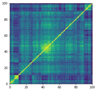
plt.figure(figsize=(5, 5))
plt.pcolormesh(corrs[0])
plt.show()
train_size = 14000
train_images = corrs[:train_size]
test_images = corrs[train_size:]
train_images = train_images.reshape(
    train_images.shape[0], n, n, 1).astype('float32')
test_images = test_images.reshape(
    test_images.shape[0], n, n, 1).astype('float32')
TRAIN_BUF = train_size
TEST_BUF = len(corrs) - train_size
BATCH_SIZE = 100
train_dataset = (tf.data.Dataset
                 .from_tensor_slices(train_images)
                 .shuffle(TRAIN_BUF)
                 .batch(BATCH_SIZE))
test_dataset = (tf.data.Dataset
                .from_tensor_slices(test_images)
                .shuffle(TEST_BUF)
                .batch(BATCH_SIZE))
class CVAE(tf.keras.Model):
    def __init__(self, latent_dim):
        super(CVAE, self).__init__()
        self.latent_dim = latent_dim
        self.inference_net = tf.keras.Sequential([
            tf.keras.layers.InputLayer(input_shape=(n, n, 1)),
            tf.keras.layers.Conv2D(
                filters=32, kernel_size=3, strides=(2, 2), activation='relu'),
            tf.keras.layers.Conv2D(
                filters=64, kernel_size=3, strides=(2, 2), activation='relu'),
            tf.keras.layers.Conv2D(
                filters=128, kernel_size=3, strides=(2, 2), activation='relu'),
            tf.keras.layers.Flatten(),
            # No activation
            tf.keras.layers.Dense(latent_dim + latent_dim),
        ])

        self.generative_net = tf.keras.Sequential([
            tf.keras.layers.InputLayer(input_shape=(latent_dim,)),
            tf.keras.layers.Dense(units=25*25*64, activation=tf.nn.relu),
            tf.keras.layers.Reshape(target_shape=(25, 25, 64)),
            tf.keras.layers.Conv2DTranspose(
                filters=128,
                kernel_size=3,
                strides=(1, 1),
                padding="SAME",
                activation='relu'),
            tf.keras.layers.Conv2DTranspose(
                filters=64,
                kernel_size=3,
                strides=(2, 2),
                padding="SAME",
                activation='relu'),
            tf.keras.layers.Conv2DTranspose(
                filters=32,
                kernel_size=3,
                strides=(2, 2),
                padding="SAME",
                activation='relu'),
            # No activation
            tf.keras.layers.Conv2DTranspose(
                filters=1,
                kernel_size=3,
                strides=(1, 1),
                padding="SAME"),
        ])

    @tf.function
    def sample(self, eps=None):
        if eps is None:
            eps = tf.random.normal(shape=(BATCH_SIZE, self.latent_dim))
        return self.decode(eps, apply_sigmoid=True)

    def encode(self, x):
        mean, logvar = tf.split(self.inference_net(x),
                                num_or_size_splits=2, axis=1)
        return mean, logvar

    def reparameterize(self, mean, logvar):
        eps = tf.random.normal(shape=mean.shape)
        return eps * tf.exp(logvar * .5) + mean

    def decode(self, z, apply_sigmoid=False):
        logits = self.generative_net(z)
        if apply_sigmoid:
            probs = tf.sigmoid(logits)
            return probs

        return logits
optimizer = tf.keras.optimizers.Adam(1e-4)

def log_normal_pdf(sample, mean, logvar, raxis=1):
    log2pi = tf.math.log(2. * np.pi)
    return tf.reduce_sum(
        -.5 * ((sample - mean) ** 2. * tf.exp(-logvar) + logvar + log2pi),
        axis=raxis)

@tf.function
def compute_loss(model, x):
    mean, logvar = model.encode(x)
    z = model.reparameterize(mean, logvar)
    x_logit = model.decode(z)

    cross_ent = tf.nn.sigmoid_cross_entropy_with_logits(logits=x_logit,
                                                        labels=x)
    logpx_z = -tf.reduce_sum(cross_ent, axis=[1, 2, 3])
    logpz = log_normal_pdf(z, 0., 0.)
    logqz_x = log_normal_pdf(z, mean, logvar)
    return -tf.reduce_mean(logpx_z + 0.03 * (logpz - logqz_x))

@tf.function
def compute_apply_gradients(model, x, optimizer):
    with tf.GradientTape() as tape:
        loss = compute_loss(model, x)
    gradients = tape.gradient(loss, model.trainable_variables)
    optimizer.apply_gradients(zip(gradients, model.trainable_variables))
epochs = 7000
latent_dim = 100
num_examples_to_generate = 16

random_vector_for_generation = tf.random.normal(
    shape=[num_examples_to_generate, latent_dim])
model = CVAE(latent_dim)
def generate_and_save_images(model, epoch, test_input):
    predictions = model.sample(test_input)
    fig = plt.figure(figsize=(16, 16))

    for i in range(predictions.shape[0]):
        plt.subplot(4, 4, i+1)
        plt.imshow(predictions[i, :, :, 0])
        plt.axis('off')

    plt.savefig('image_at_epoch_{:04d}.png'.format(epoch))
    plt.show()
generate_and_save_images(model, 0, random_vector_for_generation)

for epoch in range(1, epochs + 1):
    start_time = time.time()
    for train_x in train_dataset:
        compute_apply_gradients(model, train_x, optimizer)
    end_time = time.time()

    if epoch % 1 == 0:
        loss = tf.keras.metrics.Mean()
        for test_x in test_dataset:
            loss(compute_loss(model, test_x))
        elbo = -loss.result()
        display.clear_output(wait=False)
        print('Epoch: {}, Test set ELBO: {}, '
              'time elapse for current epoch {}'.format(epoch,
                                                        elbo,
                                                        end_time - start_time))
        generate_and_save_images(
            model, epoch, random_vector_for_generation)
Epoch: 7000, Test set ELBO: -6138.19287109375, time elapse for current epoch 48.73952054977417
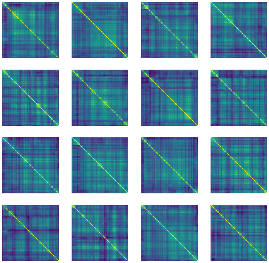
We can notice that the raw samples produced by the VAE model are optically symmetric, which was not the case with CorrGAN as displayed there.
noise = tf.random.normal(
    shape=[1, latent_dim])

predictions = model.sample(noise)

mat = np.array(predictions[0, :, :, 0])
nrm = 2 * mat - 1

plt.figure(figsize=(15, 5))
plt.subplot(1, 3, 1)
plt.pcolormesh(mat)
plt.colorbar()

plt.subplot(1, 3, 2)
plt.plot(np.diag(mat))
plt.subplot(1, 3, 3)
plt.pcolormesh(nrm)
plt.colorbar()
plt.show()
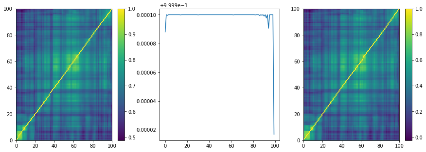
The diagonal of random samples is very close to 1 as well, which was less the case with CorrGAN as displayed there.
nb_samples = 500

generated_correls = []
for i in range(nb_samples):
    noise = tf.random.normal(shape=[1, latent_dim])
    generated_image = model.sample(noise)
    correls = 2 * np.array(generated_image[0, :, :, 0]) - 1
    generated_correls.extend(list(correls[a, b]))

empirical_correls = []
for i in range(len(corrs[:min(nb_samples, len(corrs)), :, :])):
    empirical = 2 * corrs[i, :, :] - 1
    empirical_correls.extend(list(empirical[a, b]))
len(generated_correls), len(empirical_correls)
(2475000, 2475000)
plt.hist(generated_correls, bins=100, alpha=0.5,
         density=True, label='VAE correlations')
plt.hist(empirical_correls, bins=100, alpha=0.5,
         density=True, label='empirical correlations')
plt.axvline(x=np.mean(generated_correls),
            color='b', linestyle='dashed', linewidth=2)
plt.axvline(x=np.mean(empirical_correls),
            color='r', linestyle='dashed', linewidth=2)
plt.legend()
plt.show()

plt.hist(generated_correls, bins=100, alpha=0.5,
         density=True, log=True, label='VAE correlations')
plt.hist(empirical_correls, bins=100, alpha=0.5,
         density=True, log=True, label='empirical correlations')
plt.axvline(x=np.mean(generated_correls),
            color='b', linestyle='dashed', linewidth=2)
plt.axvline(x=np.mean(empirical_correls),
            color='r', linestyle='dashed', linewidth=2)
plt.legend()
plt.show()
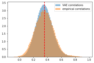

The distribution of coefficients generated by VAE matches a bit more closely the empirical distribution of estimated correlation coefficients than the one from CorrGAN as displayed there.
from statsmodels.stats.correlation_tools import corr_nearest

nb_samples = 500

generated_corr_mats = []
for i in range(nb_samples):
    print(i + 1, "/", nb_samples)

    noise = tf.random.normal(shape=[1, latent_dim])
    generated_image = model.sample(noise)
    correls = 2 * np.array(generated_image[0, :, :, 0]) - 1
    # set diag to 1
    np.fill_diagonal(correls, 1)
    # symmetrize
    correls[b, a] = correls[a, b]
    # nearest corr
    nearest_correls = corr_nearest(correls)
    # set diag to 1
    np.fill_diagonal(nearest_correls, 1)
    # symmetrize
    nearest_correls[b, a] = nearest_correls[a, b]

    generated_corr_mats.append(nearest_correls)
empirical_corr_mats = []
for i in range(len(corrs[:min(nb_samples, len(corrs)), :, :])):
    empirical = 2 * corrs[i, :, :] - 1
    empirical_corr_mats.append(empirical)
def compute_eigenvals(correls):
eigenvalues = []
for corr in correls:
eigenvals, eigenvecs = np.linalg.eig(corr)
eigenvalues.append(sorted(eigenvals, reverse=True))
return eigenvalues
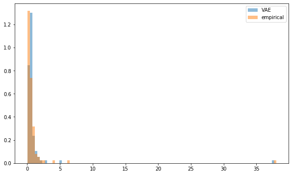
sample_mean_empirical_eigenvals = np.mean(
compute_eigenvals(empirical_corr_mats), axis=0)
sample_mean_dcgan_eigenvals = np.mean(
compute_eigenvals(generated_corr_mats), axis=0)
plt.figure(figsize=(10, 6))
plt.hist(sample_mean_dcgan_eigenvals, bins=n,
         density=True, alpha=0.5, label='VAE')
plt.hist(sample_mean_empirical_eigenvals, bins=n,
         density=True, alpha=0.5, label='empirical')
plt.legend()
plt.show()
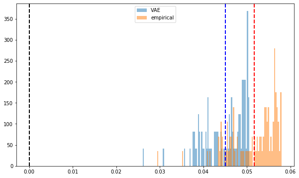
def compute_pf_vec(correls):
    pf_vectors = []
    for corr in correls:
        eigenvals, eigenvecs = np.linalg.eig(corr)
        pf_vector = eigenvecs[:, np.argmax(eigenvals)]
        if len(pf_vector[pf_vector < 0]) > len(pf_vector[pf_vector > 0]):
            pf_vector = -pf_vector
        pf_vectors.append(pf_vector)

    return pf_vectors

mean_empirical_pf = np.mean(
    compute_pf_vec(empirical_corr_mats), axis=0)
mean_dcgan_pf = np.mean(
    compute_pf_vec(generated_corr_mats), axis=0)
plt.figure(figsize=(10, 6))
plt.hist(mean_dcgan_pf, bins=n, density=True,
         alpha=0.5, label='VAE')
plt.hist(mean_empirical_pf, bins=n, density=True,
         alpha=0.5, label='empirical')
plt.axvline(x=0,
            color='k', linestyle='dashed', linewidth=2)
plt.axvline(x=np.mean(mean_dcgan_pf),
            color='b', linestyle='dashed', linewidth=2)
plt.axvline(x=np.mean(mean_empirical_pf),
            color='r', linestyle='dashed', linewidth=2)
plt.legend()
plt.show()
import fastcluster
from scipy.cluster import hierarchy
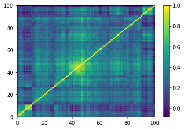
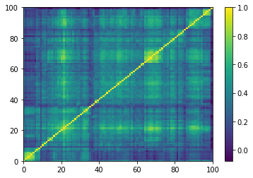
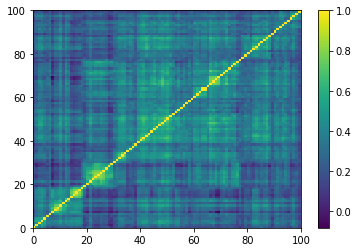
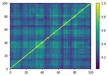
for idx, corr in enumerate(empirical_corr_mats):
dist = 1 - corr
Z = fastcluster.linkage(dist[a, b], method='ward')
permutation = hierarchy.leaves_list(
hierarchy.optimal_leaf_ordering(Z, dist[a, b]))
prows = corr[permutation, :]
ordered_corr = prows[:, permutation]
plt.pcolormesh(ordered_corr)
plt.colorbar()
plt.show()
if idx > 5:
break
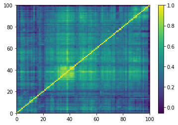
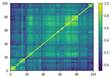
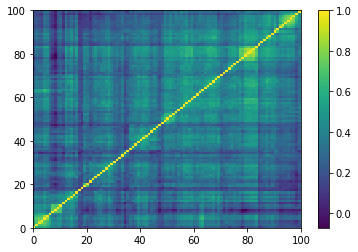
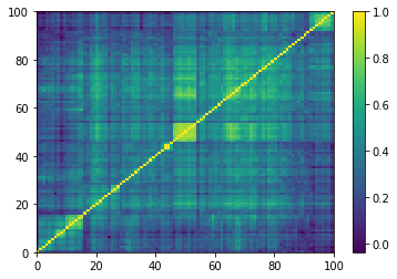
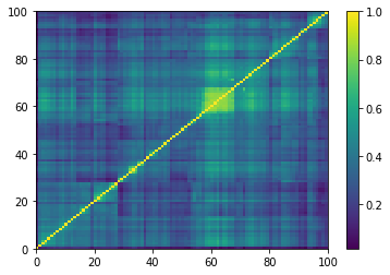
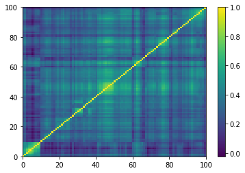
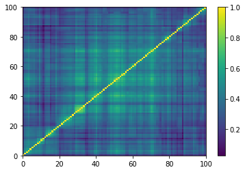
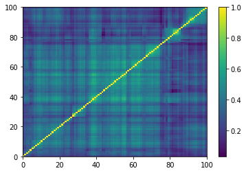
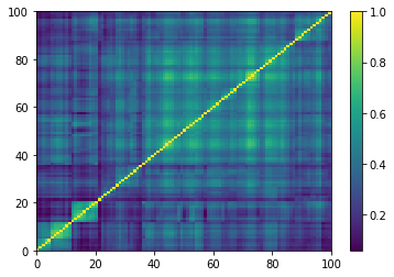
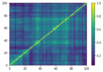
for idx, corr in enumerate(generated_corr_mats):
    # cheat: set diagonal to 1
    np.fill_diagonal(corr, 1)
    dist = 1 - corr
    Z = fastcluster.linkage(dist[a, b], method='ward')
    permutation = hierarchy.leaves_list(
        hierarchy.optimal_leaf_ordering(Z, dist[a, b]))
    prows = corr[permutation, :]
    ordered_corr = prows[:, permutation]

    plt.pcolormesh(ordered_corr)
    plt.colorbar()
    plt.show()

    if idx > 5:
        break
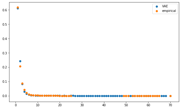
def compute_degree_counts(correls):
    all_counts = []
    for corr in correls:
        dist = (1 - corr) / 2
        G = nx.from_numpy_matrix(dist)
        mst = nx.minimum_spanning_tree(G)

        degrees = {i: 0 for i in range(len(corr))}
        for edge in mst.edges:
            degrees[edge[0]] += 1
            degrees[edge[1]] += 1
        degrees = pd.Series(degrees).sort_values(ascending=False)
        cur_counts = degrees.value_counts()
        counts = np.zeros(len(corr))
        for i in range(len(corr)):
            if i in cur_counts:
                counts[i] = cur_counts[i]

        all_counts.append(counts / (len(corr) - 1))

    return all_counts
import networkx as nx

mean_dcgan_counts = np.mean(
    compute_degree_counts(generated_corr_mats), axis=0)
mean_dcgan_counts = (pd
                     .Series(mean_dcgan_counts)
                     .replace(0, np.nan))

mean_empirical_counts = np.mean(
    compute_degree_counts(empirical_corr_mats), axis=0)
mean_empirical_counts = (pd
                         .Series(mean_empirical_counts)
                         .replace(0, np.nan))
plt.figure(figsize=(10, 6))
plt.scatter(mean_dcgan_counts.index,
            mean_dcgan_counts,
            label='VAE')
plt.scatter(mean_empirical_counts.index,
            mean_empirical_counts,
            label='empirical')
plt.legend()
plt.show()
plt.figure(figsize=(10, 6))
plt.scatter(np.log10(mean_dcgan_counts.index),
            np.log10(mean_dcgan_counts),
            label='VAE')
plt.scatter(np.log10(mean_empirical_counts.index),
            np.log10(mean_empirical_counts),
            label='empirical')
plt.legend()
plt.show()
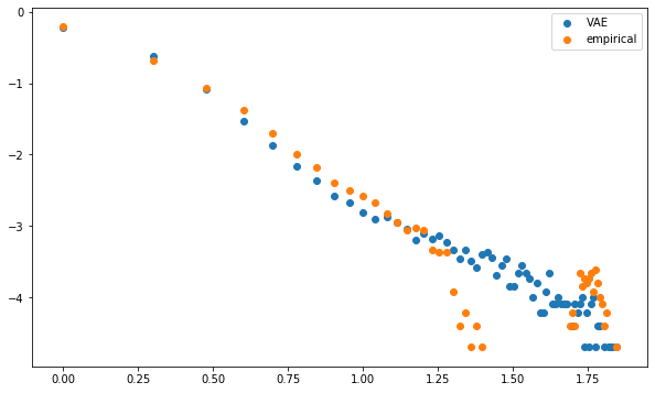
Conclusion: CorrVAE provides decent results. Need more exploration on how to balance the trade-off between reconstruction and regularization loss. How to deal with the discontinuities? Might need a major change in the model… What about a VAE with a multivariate Student instead of a multivariate Gaussian distribution?