Wasserstein Barycenters of Stocks Empirical Copulas
What’s the typical dependence between stocks?
Comparing, summarizing and reducing the dimensionality of empirical probability measures defined on a space $\Omega$ are fundamental tasks in statistics and machine learning.
Wasserstein barycenter? Briefly, it is just a mean in a metric space.
Wasserstein barycenters have a lot of interesting properties. You can have a look at the Figure 1 from the article Fast Computation of Wasserstein Barycenters, and this presentation for an intuitive understanding.
Wasserstein barycenters are one of my favourite tools when dealing with empirical distributions.
An implementation of Wasserstein barycenters is readily available in this Python library: POT: Python Optimal Transport.
In this short blog, we will simply compute the average dependence structure between two stocks. What does it look like?
%matplotlib inline

import pandas as pd
import numpy as np
from scipy.stats import rankdata
from scipy.cluster import hierarchy
import ot
import fastcluster
import matplotlib.pyplot as plt
Let’s load adjusted stock prices for names in the S&P500, and compute their returns.
df = pd.read_csv('data/SP500_HistoTimeSeries.csv')
df = df.set_index('Date')
df.index = pd.to_datetime(df.index)
df = df.sort_index()
df = df.fillna(method='ffill', limit=5)
del df['SPX Index']
returns = df.pct_change()

recent_returns = returns.iloc[-252 * 4:]

for col in recent_returns:
    try:
        if (len(recent_returns[col].dropna()) <
            len(recent_returns[col])):
            del recent_returns[col]
        if col not in industry_tickers:
            del recent_returns[col]
    except:
        pass
The sample contains 478 stocks with 1008 daily returns each (4 years of trading).
recent_returns.shape
(1008, 478)
The usual hierarchical clustering piece of code you are familiar with if you follow this blog regularly:
corr_returns = recent_returns.corr()

# sorting by hierarchical clustering
dist = 1 - corr_returns.values
dim = len(dist)
tri_a, tri_b = np.triu_indices(dim, k=1)
Z = fastcluster.linkage(dist[tri_a, tri_b], method='ward')
permutation = hierarchy.leaves_list(
    hierarchy.optimal_leaf_ordering(Z, dist[tri_a, tri_b]))
HC_tickers = recent_returns.columns[permutation]
HC_corr = corr_returns.values[permutation, :][:, permutation]

nb_clusters = 9

dist = 1 - HC_corr
dim = len(dist)
tri_a, tri_b = np.triu_indices(dim, k=1)
Z = fastcluster.linkage(dist[tri_a, tri_b], method='ward')
clustering_inds = hierarchy.fcluster(Z, nb_clusters,
                                     criterion='maxclust')
clusters = {i: [] for i in range(min(clustering_inds),
                                 max(clustering_inds) + 1)}
for i, v in enumerate(clustering_inds):
    clusters[v].append(i)

plt.figure(figsize=(5, 5))
plt.pcolormesh(HC_corr)
for cluster_id, cluster in clusters.items():
    xmin, xmax = min(cluster), max(cluster)
    ymin, ymax = min(cluster), max(cluster)

    plt.axvline(x=xmin,
                ymin=ymin / dim, ymax=(ymax + 1) / dim,
                color='r')
    plt.axvline(x=xmax + 1,
                ymin=ymin / dim, ymax=(ymax + 1) / dim,
                color='r')
    plt.axhline(y=ymin,
                xmin=xmin / dim, xmax=(xmax + 1) / dim,
                color='r')
    plt.axhline(y=ymax + 1,
                xmin=xmin / dim, xmax=(xmax + 1) / dim,
                color='r')
plt.show()
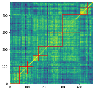
We obtain a sorted correlation matrix, with 9 clusters highlighted by the red squares.
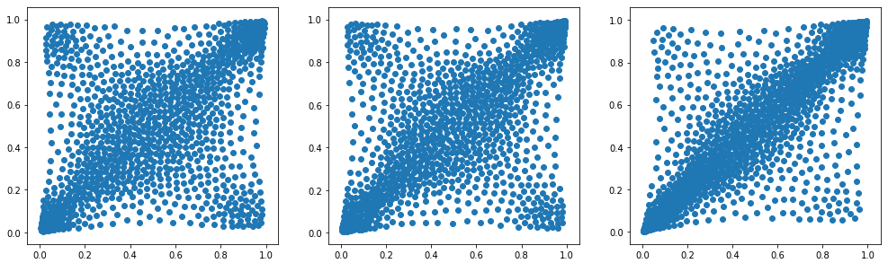
For each cluster of stocks, we compute empirical bivariate copulas between its members. From this set of bivariate distributions, we compute an average, namely a Wasserstein barycenter, which summarizes the average distribution.
mean_copula = {}
for i, cluster in enumerate(clusters):
    tickers = [HC_tickers[ind] for ind in clusters[cluster]]

    measures_locations = []
    measures_weights = []
    for id1, ticker1 in enumerate(tickers):
        r1 = recent_returns[ticker1]
        for id2, ticker2 in enumerate(tickers):
            if id2 > id1:
                    r2 = recent_returns[ticker2]
                    ranks = (pd
                             .concat([pd.Series(r1),
                                      pd.Series(r2)],
                                     axis=1, keys=['U', 'V'])
                             .dropna()
                             .rank(method='first'))
                    unifs = ranks / len(ranks)

                    measures_locations.append(unifs.values)
                    measures_weights.append(
                        np.array([1 /  len(unifs)
                                  for i in range(len(unifs))]))

    # the support for the mean will have the same number of 'diracs'
    # than the input measures
    size = len(measures_locations[0])
    X_init = np.vstack((np.random.uniform(size=size),
                        np.random.uniform(size=size))).T
    k = size
    b = np.ones((k,)) / k

    random_ids = np.random.randint(
        0, len(measures_locations),
        size=min(200, len(measures_locations)))
    locations = [measures_locations[idx]
                 for idx in random_ids]
    weights = [measures_weights[idx]
               for idx in random_ids]

    X = ot.lp.free_support_barycenter(
        locations, weights, X_init, b)

    mean_copula[i] = X
We end up with 9 barycenters, one for each cluster:
plt.figure(figsize=(17, 34))
for i in range(len(mean_copula)):
    plt.subplot(6, 3, i + 1)
    plt.scatter(mean_copula[i][:, 0],
                mean_copula[i][:, 1])

for i in range(len(mean_copula)):
    plt.subplot(6, 3, i + 9 + 1)
    hist, x_bins, y_bins = np.histogram2d(
        mean_copula[i][:, 0], mean_copula[i][:, 1], bins=25)
    plt.pcolormesh(hist)
plt.show()
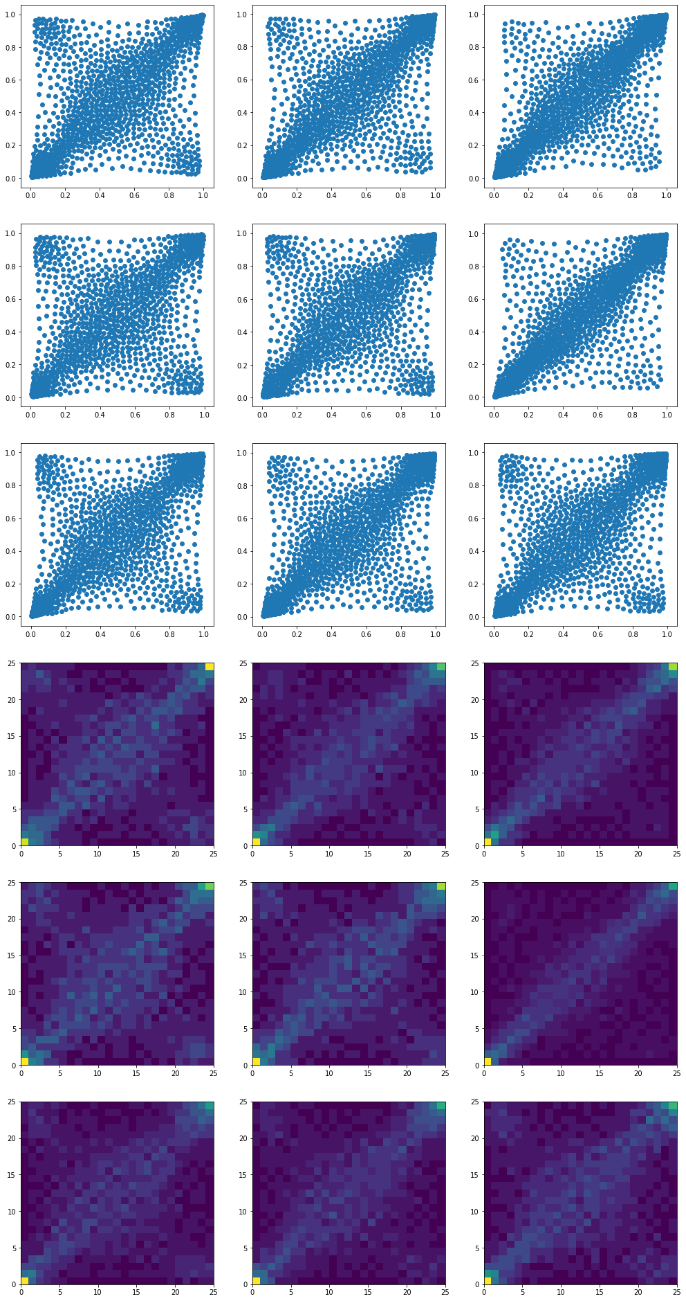
Note that many clusters exhibit anti-correlation in the extreme, i.e. extreme positive return for some stock whereas, at the same time, extreme negative return for the other.
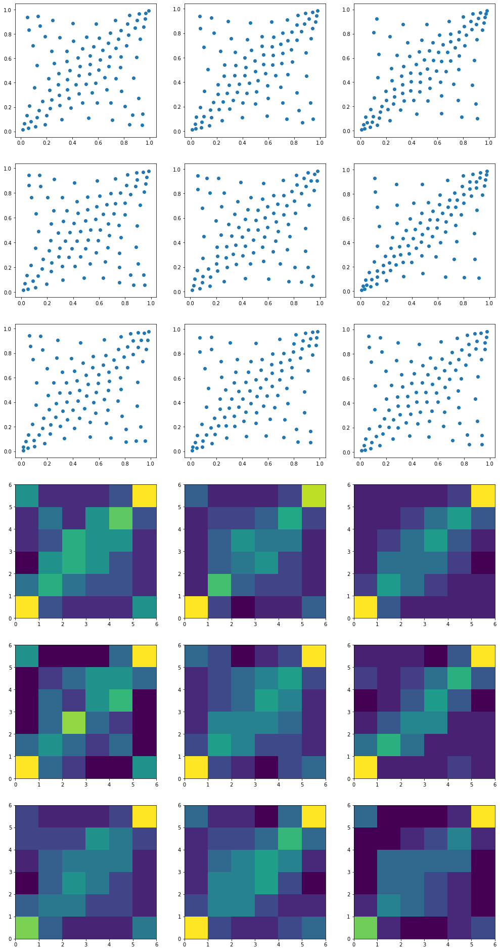
We can summarize the empirical distribution which is originally supported by 1008 ‘diracs’ with a larger or smaller support. In the example below, we re-compute the barycenters with 10 times less ‘diracs’. The shape of the distribution is the same, but an estimation of density would be much harder as you can see below…
mean_copula_small_support = {}
for i, cluster in enumerate(clusters):
    tickers = [HC_tickers[ind] for ind in clusters[cluster]]

    measures_locations = []
    measures_weights = []
    for id1, ticker1 in enumerate(tickers):
        r1 = recent_returns[ticker1]
        for id2, ticker2 in enumerate(tickers):
            if id2 > id1:
                    r2 = recent_returns[ticker2]
                    ranks = (pd
                             .concat([pd.Series(r1),
                                      pd.Series(r2)],
                                     axis=1, keys=['U', 'V'])
                             .dropna()
                             .rank(method='first'))
                    unifs = ranks / len(ranks)

                    measures_locations.append(unifs.values)
                    measures_weights.append(
                        np.array([1 /  len(unifs)
                                  for i in range(len(unifs))]))

    # the support for the mean will have M times less 'diracs'
    # than the input measures
    M = 10
    size = int(len(measures_locations[0]) / M)
    X_init = np.vstack((np.random.uniform(size=size),
                        np.random.uniform(size=size))).T
    k = size
    b = np.ones((k,)) / k

    random_ids = np.random.randint(
        0, len(measures_locations),
        size=min(200, len(measures_locations)))
    locations = [measures_locations[idx]
                 for idx in random_ids]
    weights = [measures_weights[idx]
               for idx in random_ids]

    X = ot.lp.free_support_barycenter(
        locations, weights, X_init, b)

    mean_copula_small_support[i] = X
plt.figure(figsize=(17, 34))
for i in range(len(mean_copula_small_support)):
    plt.subplot(6, 3, i + 1)
    plt.scatter(mean_copula_small_support[i][:, 0],
                mean_copula_small_support[i][:, 1])

for i in range(len(mean_copula_small_support)):
    plt.subplot(6, 3, i + 9 + 1)
    hist, x_bins, y_bins = np.histogram2d(
        mean_copula_small_support[i][:, 0],
        mean_copula_small_support[i][:, 1],
        bins=6)
    plt.pcolormesh(hist)
plt.show()
In future short blogs,
- we will sample from these copula barycenters,
- we will try to find stylized facts,
- we will check the margins cluster by cluster, and summarize them with Wasserstein barycenters,
- we will sample synthetic bivariate returns (using the copula and the two margins).
From this basic knowledge gained from the data, we will try to develop and benchmark CopulaGAN (for sampling in higher dimensions, where histogram-based methods fall short).