Embeddings of Sectors and Industries using Graph Neural Networks
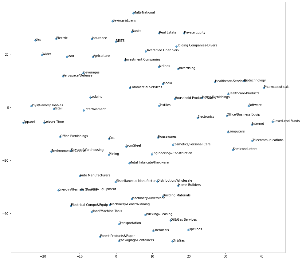 node2vec embeddings of industries projected onto the 2d plane
Embeddings of Sectors and Industries using Graph Neural Networks
You can find the reproducible experiment in this Colab Notebook.
In econometrics and financial research, categorical variables, and especially sectors and industries, are usually encoded as dummy variables (also called one-hot encoding in the machine learning community). You can find plenty of such examples in the SSRN literature, where authors are regressing the performance of their signal on standard factors such as value, quality, size, momentum, sectors and industries to demonstrate that their signal is adding value (statistically significant alpha > 0) on top of the well-known standard factors.
Let’s illustrate more concretely what the one-hot encoding means: If we consider the possible sectors (Utilities, Technology, Transportation) and the industries (Airlines, Internet, Eletric, Gas), the one-hot encoding for the following companies (Google, Dynegy, Amazon, New Jersey Resources, Delta Air Lines) is the following:
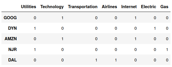
dummy variables (one-hot encoding) for sector, industry
However, such one-hot encoding does not take into account that some industries are closer to each other (say Electric and Gas) than to some others (say Internet). When embedded in the ambient Euclidean space, one-hot encoded industries are all equidistant to each other at a distance of $\sqrt{2}$. We know that some industries have strong supply chains ties, and interdependent businesses (think Auto Manufacturers and Auto Parts & Equipment). Looking at the correlation matrix of industry returns confirms this narrative.
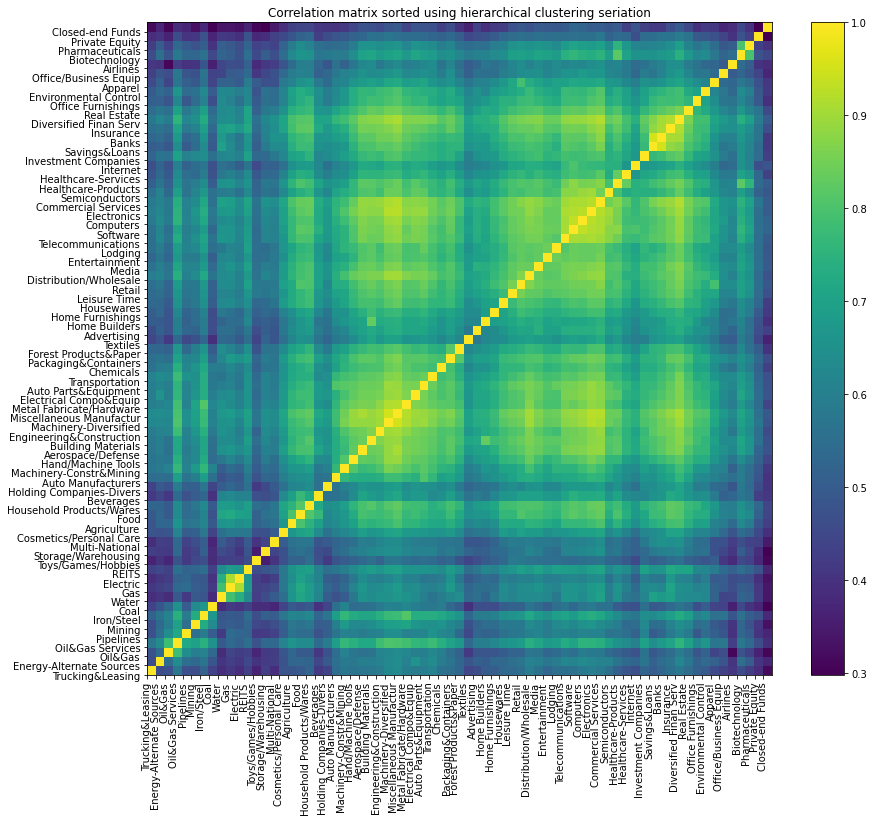 correlation matrix between industries
Transforming one-hot encodings into continuous vectors is by now a very common knowledge and standard practice of deep learners (e.g. word2vec). Embeddings obtained using neural networks were shown to exhibit nice properties which could be intuitively understood: For example, vec(“Russia”) + vec(“river”) is close to vec(“Volga River”), and vec(“Germany”) + vec(“capital”) is close to vec(“Berlin”). One of the main basic idea to obtain these embeddings is to use self-supervision: Given the data, use some pieces to predict the rest. This is basically the idea of the Skip-gram model in word2vec (natural language processing) which aims to find word representations that are useful for predicting the surrounding words in a sentence or a document. More recently, these embeddings (neural networks) techniques were extended to graphs (e.g. 3D models of proteins, social networks, knowledge graphs). Using these embeddings has been shown to boost results in downstream tasks such as more accurate predictions (e.g. a better recommender system).
Since this idea is not yet well known and explored in the econometrics and financial research literature, we describe a simple use case in this blog: embeddings of sectors and industries using one of the most vanilla technique (node2vec) with very standard non IP-sensitive data: US stocks returns and their correlations.
We won’t explore downstream tasks (e.g. regressions) in this blog. However, we expect that using these continuous embeddings instead of dummy variables can help regressions by increasing data efficiency (i.e. one needs less data to fit the model, or one gets better performance for the same amount of data): We can leverage the data points in one industry to help predictions on another very similar industry (located closely in the embedding space). The latter property being especially important in finance where the number of data points is usually too small (with respect to the amount of data needed to obtain stable models (e.g. Random Matrix Theory and the estimation of covariance matrices) or statistically valid results) for many interesting problems at hand. We leave for a future blog-experiment to test this intuition on a non-IP sensitive regression.
Summary of the approach implemented in this blog:
In this blog, we consider US stocks, their industry (according to some classification which doesn’t matter; You could repeat the experiment with statistical clusters as described in this old blog: Study of US Stocks Correlations, Hierarchies and Clusters).
-
We (naively) obtain an industry return time series by averaging the returns of all the stocks which belong to that industry.
-
We compute the industry correlation matrix
-
We compute a network out of this correlation matrix (cf. How to compute the Planar Maximally Filtered Graph (PMFG))
-
We apply node2vec using the StellarGraph library
-
We evaluate qualitatively the embeddings obtained by projecting them on the 2D plane with t-SNE
TL;DR Using continuous embeddings of sectors and industries obtained with various graph neural networks techniques may help improve the results of downstream tasks (e.g residualisation of a signal, regression $R^2$) instead of encoding this information as a dummy variable (one-hot encoding) as usually done in the econometrics and financial research literature.
import numpy as np
import pandas as pd
import planarity
import networkx as nx
from scipy.cluster import hierarchy
from sklearn.manifold import TSNE
from stellargraph.data import BiasedRandomWalk
from stellargraph import StellarGraph
from gensim.models import Word2Vec
from tqdm import tqdm
import matplotlib.pyplot as plt
stock_features = pd.read_csv(
    'https://sp500-histo.s3.ap-southeast-1.amazonaws.com/stock_features.csv')
stock_features['INDUSTRY_GROUP'].value_counts().plot(kind='bar',
                                                     figsize=(24, 6))
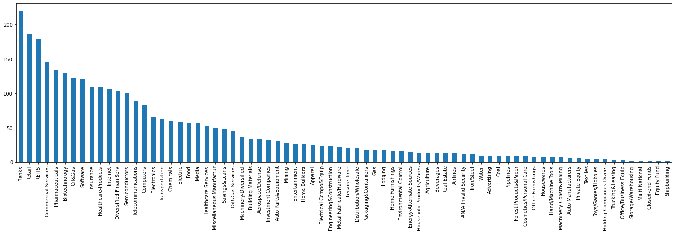 number of US stocks per industry
tickers_sectors = stock_features[['Unnamed: 0', 'INDUSTRY_GROUP']]
tickers_sectors.columns = ['ticker', 'industry']
tickers_sectors = tickers_sectors[
    tickers_sectors.industry != '#N/A Invalid Security']
tickers_sectors.sort_values('industry')
| ticker | industry | |
|---|---|---|
| 2726 | SZMK | Advertising |
| 1837 | MM | Advertising |
| 1767 | MCHX | Advertising |
| 2093 | OMC | Advertising |
| 2839 | TRMR | Advertising |
| ... | ... | ... |
| 764 | CWT | Water |
| 3123 | WTR | Water |
| 1885 | MSEX | Water |
| 282 | AWR | Water |
| 3164 | YORW | Water |
3178 rows × 2 columns
stock_prices = pd.read_csv(
    'https://sp500-histo.s3.ap-southeast-1.amazonaws.com/WIKI_PRICES.csv')
df_prices = pd.pivot(stock_prices[['ticker', 'date', 'adj_close']],
                     index='date', columns='ticker', values='adj_close')
del stock_prices

recent_returns = df_prices.pct_change().iloc[-2000:]
selected_columns = []
for col in tqdm(df_prices.columns):
  if len(recent_returns[col].dropna()) > 0.98 * len(recent_returns[col]):
    selected_columns.append(col)
100%|██████████| 3190/3190 [00:00<00:00, 5821.53it/s]
len(selected_columns)
2589
df_returns = recent_returns[selected_columns].fillna(0)
stacked_returns = df_returns.stack().reset_index()
stacked_returns.columns = ['date', 'ticker', 'return']
ticker_sector_returns = pd.merge(
    tickers_sectors, stacked_returns, on=['ticker'])
mean_return_industry = (ticker_sector_returns
                        .groupby(['industry', 'date'])['return']
                        .mean()
                        .clip(lower=-0.25, upper=0.25)
                        .reset_index())
df_industry_returns = pd.pivot(mean_return_industry,
                               index='date',
                               columns='industry',
                               values='return')
df_industry_returns.cumsum().plot(figsize=(24, 6), legend=False)
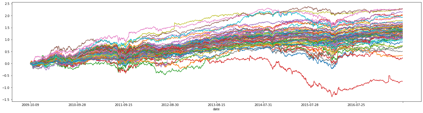 time series of the industries returns
df_industry_returns.stack().hist(bins=100, log=True)
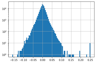
distribution of the industries daily returns
# sorted by hierarchical clustering
corr_returns = df_industry_returns.corr()

dist = 1 - corr_returns.values
dim = len(dist)
tri_a, tri_b = np.triu_indices(dim, k=1)
Z = hierarchy.linkage(dist[tri_a, tri_b], method='ward')
permutation = hierarchy.leaves_list(
    hierarchy.optimal_leaf_ordering(Z, dist[tri_a, tri_b]))

HC_tickers = df_industry_returns.columns[permutation]
HC_corr = corr_returns.values[permutation, :][:, permutation]
corr = pd.DataFrame(HC_corr, columns=HC_tickers, index=HC_tickers)

plt.figure(figsize=(14, 12))
plt.pcolormesh(corr)
plt.colorbar()
plt.title('Correlation matrix sorted using hierarchical clustering seriation')
plt.xticks(ticks=range(len(corr)),
           labels=corr.columns,
           rotation=90)
plt.yticks(ticks=range(len(corr)),
           labels=corr.columns)
plt.show()
correlation matrix between industries
Computing the PMFG from the correlation matrix
cf. previous blog How to compute the Planar Maximally Filtered Graph (PMFG)
cf. literature review: A review of two decades of correlations, hierarchies, networks and clustering in financial markets
def sort_graph_edges(G):
    sorted_edges = []
    for source, dest, data in sorted(G.edges(data=True),
                                     key=lambda x: x[2]['weight']):
        sorted_edges.append({'source': source,
                             'dest': dest,
                             'weight': data['weight']})

    return sorted_edges


def compute_PMFG(sorted_edges, nb_nodes):
    PMFG = nx.Graph()
    for edge in sorted_edges:
        PMFG.add_edge(edge['source'], edge['dest'])
        if not planarity.is_planar(PMFG):
            PMFG.remove_edge(edge['source'], edge['dest'])

        if len(PMFG.edges()) == 3*(nb_nodes-2):
            break

    return PMFG

complete_graph = nx.Graph()
for i in range(len(corr)):
    for j in range(i+1, len(corr)):
        complete_graph.add_edge(corr.columns[i],
                                corr.columns[j],
                                weight=1 - corr.values[i, j])

sorted_edges = sort_graph_edges(complete_graph)

PMFG = compute_PMFG(sorted_edges, len(complete_graph.nodes))
edges = list(PMFG.edges)

list_edges = []
for edge in edges:
  list_edges.append((edge[0],
                     edge[1],
                     corr.loc[edge[0]][edge[1]]))
edges = pd.DataFrame(list_edges)
edges.columns = ['source', 'target', 'weight']
edges
| source | target | weight | |
|---|---|---|---|
| 0 | Machinery-Diversified | Miscellaneous Manufactur | 0.951372 |
| 1 | Machinery-Diversified | Electronics | 0.923191 |
| 2 | Machinery-Diversified | Metal Fabricate/Hardware | 0.915317 |
| 3 | Machinery-Diversified | Commercial Services | 0.911704 |
| 4 | Machinery-Diversified | Engineering&Construction | 0.901262 |
| ... | ... | ... | ... |
| 202 | Internet | Closed-end Funds | 0.481486 |
| 203 | Oil&Gas | Pipelines | 0.641384 |
| 204 | Advertising | Airlines | 0.529009 |
| 205 | Mining | Coal | 0.631481 |
| 206 | Holding Companies-Divers | Private Equity | 0.461794 |
207 rows × 3 columns
Application of node2vec (from StellarGraph) on the PMFG extracted from the industry correlation matrix
I played with StellarGraph for the past few months with Thomas Graff on some side project. We experimented with the Attri2Vec algorithm (graph nodes can have a rich set of features). In this blog however, we stick to a very simple vanilla algorithm: node2vec. node2vec is a direct extension of the word2vec idea by using random walks as sentences fed to the skip-gram model: “Given a word, predict its neighboring words” becomes “Given a node, predict its neighboring nodes (in the random walk)”.
G = StellarGraph(edges=edges)
print(G.info())
StellarGraph: Undirected multigraph
 Nodes: 71, Edges: 207

 Node types:
  default: [71]
    Features: none
    Edge types: default-default->default

 Edge types:
    default-default->default: [207]
        Weights: range=[0.461794, 0.951372], mean=0.786456, std=0.105644
        Features: none
rw = BiasedRandomWalk(G)
weighted_walks = rw.run(
    nodes=G.nodes(),
    length=100,
    n=50,
    p=0.5,
    q=2.0,
    weighted=True,
    seed=42)

print("Number of random walks: {}".format(len(weighted_walks)))
Number of random walks: 3550
weighted_model = Word2Vec(
    weighted_walks, size=50, window=5, min_count=0, sg=1, workers=1, iter=1
)
emb = weighted_model.wv["Beverages"]
emb.shape
(50,)
node_ids = weighted_model.wv.index2word
weighted_node_embeddings = (
    weighted_model.wv.vectors
)

tsne = TSNE(n_components=2, random_state=42)
weighted_node_embeddings_2d = tsne.fit_transform(weighted_node_embeddings)
fig, ax = plt.subplots(figsize=(16, 15))
ax.scatter(
    weighted_node_embeddings_2d[:, 0],
    weighted_node_embeddings_2d[:, 1],
    cmap="jet",
    alpha=0.7)

for i, industry in enumerate(node_ids):
    ax.annotate(industry,
                (weighted_node_embeddings_2d[i, 0],
                 weighted_node_embeddings_2d[i, 1]))
node2vec embeddings of industries projected onto the 2d plane
Conclusion: It seems that the embeddings obtained in $R^{50}$, and computed with the node2vec algorithm are sensible: When industries are projected to $R^{2}$ from $R^{50}$, their relative position matches well with the intuitive understanding of their relation to other industries.